Stormwater Best Management Practices in an Ultra-Urban Setting: Selection and Monitoring
4.4 Monitoring Program Design Phase
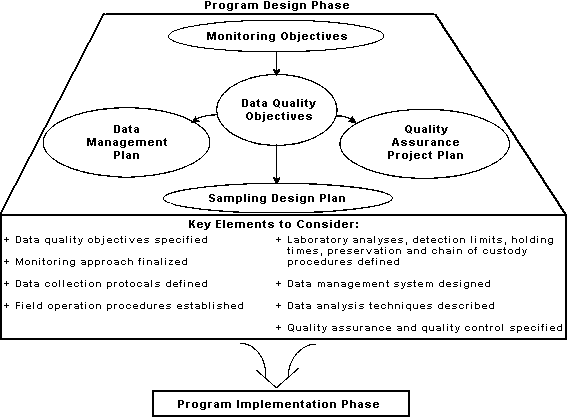
The design phase of a monitoring program for BMP evaluation is initiated following the identification of program objectives in the planning phase of the program. Components of the program design phase involve development of (1) data quality and monitoring objectives; (2) a sampling design plan, including detailed specifications for standard operating procedures, and a logistical and training program; (3) a data management plan; and (4) a Quality Assurance Project Plan (QAPP). Figure 40 illustrates the components of monitoring design and outlines the key elements to consider prior to the implementation of data collection. These components and their elements define the type and quality of data needed for a BMP performance and evaluation assessment. The design phase provides complete documentation of the data collection procedures and the rationale or justification supporting the various planning and design decisions.
Data quality objectives (DQOs) are developed and used to support preparation of a scientific and resource-effective sampling design plan (USEPA, 1994b). DQOs are qualitative or quantitative statements that clarify the monitoring program objectives, define the most appropriate type of data to collect, determine the most appropriate conditions under which to collect the data (temporal and spatial), and specify limits on decision errors that will be used to establish the quantity and quality of data needed to support the decision.
The purpose of collecting data is to answer specific management questions regarding whether a particular BMP provides a desired level of stormwater management, to evaluate differences in the constituent removal efficiencies of BMP design alternatives, or to assess the factors affecting the operation and maintenance requirements of BMPs. Specific hypotheses to be tested are usually identified during the development of monitoring objectives in the planning phase of the project. Examples of such hypotheses might include the following:
- Comparing BMP alternative designs to address specific site conditions.
No significant difference between BMP (grassed swale) design A and design B, or can BMP design A, given specific site conditions, achieve a higher constituent removal than design B?
- Comparing BMP alternative designs to address a specific constituent type.
No significant difference between the influent/effluent concentration of a given constituent for BMP design A, or can a modification or retrofit to BMP design A effectively remove a given constituent?
- Comparing various BMP types to address specific constituent loadings.
No significant differences in constituent loading reductions measured between BMP types A, B, and C (Which BMP type is most effective at reducing the loadings of a constituent?).
No significant difference in constituent removal efficiency of BMP design A with increased hydraulic/constituent loading conditions (Does BMP design A work the same under all combinations of stormwater flows and constituent loads?).
- Comparing effectiveness of BMP types or BMP designs based on downstream impacts.
No significant differences in the ability of BMP design A, B, or C to protect downstream aquatic or riparian resources (Can BMP design A, B, or C prevent downstream impacts on aquatic or riparian communities and streambank stability due to hydrologic alterations/changes?).
Illustrations of the first two hypotheses are provided in the boxes below. The design phase of the monitoring program includes the refinement of the type, quantity, and quality of the data required to support stormwater management decisions. Examples of these are:
-
BMP design A needs to be structurally modified to improve its removal efficiency for a given constituent.
-
The BMP design is reducing the loadings of constituent and can be used at other similar sites.
-
BMP design B can be used only at sites with a limited range of flows.
-
Structural modification B cannot be used to improve the removal efficiency at a retrofit site with MP design A.
Common management questions regarding ultra-urban stormwater management with respect to BMP monitoring may include a combination of the above hypotheses with emphasis on whether a particular BMP can reduce the loadings of constituents to water bodies. Measurement of constituents such as TSS, BOD, COD, nutrients (particulate and soluble fractions of nitrogen and phosphorus), and pH, as well as oil and grease, and when desired, specific chemical constituents such as the heavy metals lead, copper, zinc, and cadmium, will provide information that can be used to judge the effectiveness of the BMP design or implementation.
When multiple objectives for evaluating a BMP are considered, they may consist of establishing various constraints and an optimization scheme to assess design alternatives that will best meet management goals. An illustrative example might include control of all flows exceeding stream bankfull flow rates that have a detention of more than X hours, while preserving water temperature at lower than 18.3ºC (65ºF).
|
Comparison of Grassed Swales
A grassed swale on U.S. Route 29 south of Charlottesville, Virginia (29S) was monitored for its ability to remove constituents from highway runoff (Yu and Kaighn, 1995). This site was chosen because its characteristics contrasted with a swale on U.S. Route 29 north of Charlottesville (29N), which had been the subject of previous evaluations. The 29N swale had a slope of approximately 5 percent, whereas the 29S swale had a slope closer to 2 percent. The average daily traffic (ADT) of the 29N site was approximately 50,000, with the ADT at the 29S site approximately 30,000. Mowing was much more frequent at the 29N swale, occurring about once every 2 weeks during the growing season, while the 29S swale was mowed only four times during the same period. According to the literature, these differences should have led to higher removal efficiencies for the 29S swale.
The results of the monitoring program for the 29S swale found significantly lower constituent removals. Though lateral barriers had been installed to eliminate lateral inflow to the swale, the measured flow increased from the inflow point to the outflow point for two of the storms, resulting in negative mass balance removal results. Even if these two storms were omitted, constituent removal percentages were all less than 30 percent (significantly less than the 80-90 percent removal observed at the 29N site).
The only advantage the 29N site had over the 29S site was the downstream weir, which acted as a check dam. A significant amount of water ponded behind the weir, creating a small detention pond where constituents were allowed to settle and stormwater runoff could infiltrate into the soil. The 29N site had significant decreases in flow; it can only be assumed that this flow loss was a direct consequence of the downstream weir.
|
|
Modified Detention Pond
A dry detention pond was the focus of a recent study in Charlottesville, Virginia, (Yu et al., 1993, 1994). The immediate drainage basin for the pond is a parking facility for daily commuters and athletic event traffic. The entire watershed contributing to the detention pond is approximately 3.2 ha (7.9 ac) in size, with 60 percent of the drainage area consisting of the paved parking facility. The detention pond was initially designed and constructed solely to attenuate the post development peak runoff flow rate to the predevelopment flow rate for 2- and 10-year storms. No provisions were made for water quality improvements. To create an extended detention dry pond for water quality improvement, the outlet structure was modified to provide a slow release of the runoff from a designated storm (i.e., 2-year frequency or less). For this study, the outlet was restricted to a 7.6 cm (3 in) diameter orifice.
The first two storms where both flow and concomitant pollutant concentrations were monitored provided a baseline study of the efficiency of the existing pond, since the orifice was not in place; however, the last two storms of Phase I were monitored with the extended detention orifice in place. In Phase II, four storms were monitored for both flow and pollutant concentration. Detention time is usually considered to be one of the most important factors affecting pollutant removal; however, it appears that it is not the only determinant of pond efficiency. The two storms with paired inflow/outflow data that occurred prior to the modification of the outlet orifice had unusually high removal efficiencies. The storms were very low-intensity, low-volume storms. It is likely that the conveyance channel and the low flow conditions in the pond were sufficient enough to reduce the pollutant loads regardless of the relatively low detention time. The removal efficiencies calculated after the modification of the orifice were substantially lower than those before modification. The storms monitored following the installation of the smaller orifice produced larger runoff volumes and pollutant loads.
|
Another key step of DQO development is to identify the quantity of data needed to support the analysis and evaluation of BMPs. The "quantity of data" should address how many samples need to be analyzed from different locations and at different times, as well as how many samples need to be analyzed at each site and time, to provide estimates of sampling design error and measurement error. Should water quality parameters be measured before the BMP is implemented to provide a "before-and-after" comparison, and if so, should these measurements be taken under the same or different conditions? How many samples will be required to provide the best estimate of nutrient concentrations before and after and increase the power of statistically detecting differences between the two scenarios? How many and what kind of samples (e.g., flow-weighted during events or grab during baseflow conditions) are needed to evaluate the quality of the measurements? What analyses will be performed on the data collected (e.g., comparisons between sites or times, or among several BMPs), and how will those analyses affect the number of samples needed?
A determination of the number of samples and constituents to be analyzed should consider the resources available and cost and time constraints, as well as the quality assurance and quality control requirements to be followed to ensure that sampling design and measurement errors are controlled sufficiently to reduce uncertainty and meet the tolerable decision error rates. Several iterations of the DQO process might be required to determine the optimal sample size for different sampling design plans.
Sampling design plans are developed to test specific hypotheses and can be approached in a variety of ways. Elements of plan include (1) an evaluation of approaches to development of sampling design plans; (2) the data collection process and its associated components of site selection, sampling and sensor locations, sampling frequency and type, and sampling data representativeness; (3) equipment needs and selection; and (4) field measurements and sampling methods.
Monitoring Design Approaches
Two commonly used methods to evaluate the constituent removal effectiveness of a BMP are influent-effluent constituent monitoring and the watershed monitoring approach. An influent and effluent monitoring approach is normally confined to the BMP, whereas the watershed approach evaluates the effectiveness of either a structural or nonstructural BMP program distributed within the watershed. Examples of watershed approaches include upstream-downstream, before and after, and paired watershed (Coffey et al., 1993).
BMP Influent-Effluent Approach. The influent/effluent approach is a method of estimating the pollutant removal efficiency of an individual BMP or a series of in-line BMPs. In this approach, the effectiveness of the BMPs is isolated and a mass balance method is usually used to estimate pollutant removal efficiency. In general, pollutant removal efficiencies are based on calculating the difference between influent and effluent loads (Urbonas, 1994). There are several key benefits in applying the influent-effluent approach for BMP efficiency, which include:
- The approach is easily used to evaluate existing BMPs, particularly when the effect of BMP age is a management concern.
- The cost of monitoring is substantially less than that for some watershed approaches since not all environmental factors have to be monitored separately and factored into the overall efficiency.
- The time needed for monitoring can be substantially less than that required for watershed approaches since a specified calibration period is not necessary prior to beginning a monitoring program.
- The evaluation results for a particular type of BMP can be extrapolated to other physiographic regions as long as climate is not a major factor affecting the efficiency.
A drawback to the influent-effluent approach is the difficulty of establishing the downstream benefits of BMP implementation without additional data collection; for example, effectiveness in reducing the impacts of stormwater discharges on aquatic or riparian communities, and streambed and bank stability, due to hydrologic alterations.
Watershed Approaches. Watershed approaches to BMP evaluation are used when the physical constraints of a site do not permit adoption of an influent/effluent approach, or in the case of evaluation of the effectiveness of wide-scale application of a number of structural BMPs within a watershed. A watershed approach can also be used to evaluate the effectiveness of nonstructural BMPs such as streetsweeping, catch basin cleaning programs, the use of catch basin inserts, and public outreach programs that promote a range of methods to reduce constituent loadings in stormwater. Three commonly used watershed approaches are upstream-downstream, before and after, and paired watershed.
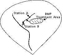
Upstream-Downstream Approach. In contrast to the influent-effluent method, the upstream/ downstream method entails a comparison of data collected from instream locations both upstream and downstream of a BMP program or structure. Monitoring at the upstream location accounts for incoming pollutant sources that are unrelated to the land treatment within the study area. This method is more complex because the BMP is no longer isolated, but rather its effectiveness must be factored into other naturally occurring climatic and environmental conditions. For example, this method must take into account the addition of tributaries between the two data collection points, as well as changes in geology. Nonetheless, if this method of monitoring is conducted properly, the results produce clear and essentially irrefutable evidence of BMP influence on the study watershed (Coffey et al., 1993). Figure 41 shows a schematic of an upstream/downstream BMP monitoring design. Station A is sited to monitor the instream concentration of constituents upstream of the land treatment area; station B is sited below the BMP treatment area.
Because of the complex influences that can result from the area between the upstream and downstream monitoring locations, as well as the condition and size of the instream water body, some researchers feel the upstream/downstream approach may not be as effective in detecting changes. The time period over which to extend a sampling program is another important issue that has to be resolved. Year-to-year and seasonal variability in water quality constituent concentrations under certain conditions may surpass the changes contributed to by the BMP over any given time period. To account for some of this variability, a monitoring period of at least two to three years is recommended for both pre- and post-BMP evaluations.
Before and After Approach. The before and after approach requires that baseline data be collected prior to implementation of a watershed-wide BMP program. Year-to-year and seasonal differences also affect this approach, and as in the upstream/downstream approach to monitoring, a two to three year pre- and post-BMP monitoring period is recommended to account for this variability (Coffey et al., 1993). The effect of longer term climatic trends on hydrologic variability may still, however, mask the removal effectiveness of a BMP program. Once the BMPs are implemented, an additional shortcoming of this approach is that the baseline data characterization cannot be improved upon. To substantiate a cause-and-effect relationship, the predictor variable should be adjusted for year-to-year changes in hydrologic conditions. Because of these problems, some experts prefer to combine this method with that of the upstream/downstream approach to strengthen the results of the findings (Coffey et al., 1993). Because hydrologic variabilities can occur over longer periods of time, comparative analysis of data collected using a before and after approach over the short term may be dealing with two distinct populations of hydrologic conditions.
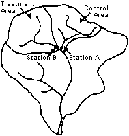
Paired Watershed Approach. The paired watershed approach entails the comparison of water quality data from two or more watersheds with at least one regarded as the control (undisturbed) watershed. Data are from concurrent time periods, and any change in these data is taken as being indicative of BMP influence. If properly implemented, this method provides reliable results and is perhaps the most effective design for monitoring BMP program effectiveness (Coffey et al., 1993). A limitation of this approach is that the watersheds compared must be in close proximity for climatic homogeneity, with similar geology and stable land uses over the study period.
Data Collection Protocols
Data collection procedures are in large part dictated by the selection of constituents to be monitored and by the data quality objectives set for the sampling program. The expected range of concentrations at which the expected constituents may be detected and the need for auxiliary information such as continuous discharge, pH, temperature, and dissolved oxygen are also important elements of data collection procedures. The availability of staff and resources to complete the data collection must also be considered.
Elements of data collection include the selection of sampling site locations, sampling methods (manual, automated), number of events sampled, and the number of samples collected during both event and baseline conditions.
Sampling Site Location. The approach selected for BMP evaluation and a range of field constraints must be considered in the installation of monitoring equipment. Proposed locations must be representative of both the inflows and outflows, and of water quality from the BMP structure when warranted. Similar requirements must also be met by instream sampling locations when the design involves watershed scale assessments of BMPs. Manual sampling programs require that the equipment used for collecting samples be capable of safely reaching representative sampling locations (points) for the range of expected flows. Access to the site and the safety of the sampling crew should be considered and given first priority.
In an ultra-urban setting, the location of utilities and other underground facilities may also need to be established before equipment installation. If automated equipment is to be installed permanently at the site, the proximity of an electrical power supply might be an important consideration. If constituents selected for monitoring have short holding times, refrigerated sampling units could be required and alternatives for transport to the laboratory should be evaluated accordingly.
In the selection of monitoring locations to install equipment shelters or for the installation of primary measuring devices such as weirs or flumes, it is necessary to secure the required permission from landowners and any government agencies that have jurisdiction over the land or waterway where equipment will be installed.
A shelter used for housing water quality sampling equipment should be easily and safely accessible, at a location that will not flood during large storm events.
Sampling and Sensor Locations. If an in situ stage-discharge relationship (rating curve) is to be developed, the stage sensor should be located along a straight stretch of channel at least 20 channel widths below any upstream bends. The bottom of the channel also needs to be relatively even and the channel configuration sensitive to changes in discharge. The stage sensor for primary measuring devices should be located as per the recommendations of the manufacturer.
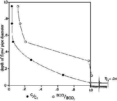
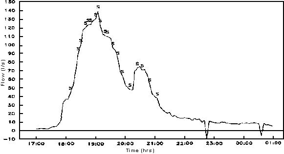
The intake line for water quality sampling should be in a well-mixed portion of the main body of the flow path. As a general rule to prevent the sampling of bedload, the intake line for an instream location needs to be placed 100-200 mm (4-8 in) above the bottom of the streambed. The actual position should be verified following equipment installation and testing in the implementation phase. For flows with depth greater than 0.76 m (2.5 ft), it also advisable to develop a relationship between the parameters sampled using a single-point automated sampler with that obtained from a hand-held depth integrating sampler such as the hand-held DH-48 (USGS, 1977). Some parameters-in particular, suspended sediment and total phosphorus-can be transported at different concentrations within the water column profile. A sampler intake located at a single point may not accurately reflect an integrated concentration (laterally and vertically) for some pollutants. The results shown in Figure 43 illustrate the concentration gradient with depth that can occur for suspended sediments and BOD5 transported in a storm drain pipe. Samples collected in the lower portion of flow (e.g., automated samplers) may result in above average concentration while, conversely, samples (i.e., grab samples) collected in the upper portion of flow would yield below average concentrations. For other flows and constituents these concentration gradients are likely to be different. It is recommended that sample intake lines be located at a cross-section where flow is turbulent (e.g., close to lateral inflows or vertical drops; Marsalek, 1973).
|
|
η=relative elevation above the sewer bottom (el. above bottom/depth of flow).
C=concentration of suspended solids (mg/l) measured at elevation η.
Cr=Concentration of suspended solids measured at ηr.
ηr=reference relative elevation (=0.04).
BODr=biochemical oxygen demand (5 day) at ηr. |
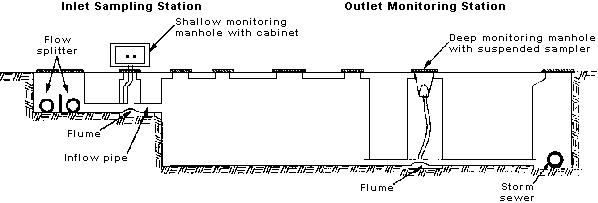
The sampling station location and sensor placement for an in/out approach for evaluation of an ultra-urban BMP is illustrated in Figure 44. The sampling station located at the inlet illustrates the placement of a monitoring station aboveground, while the outlet station shows the placement of a portable, integrated flow and water sampling equipment station inside an access hole. Water sampling lines and stage sensors for both stations are both placed within a primary flow measurement structure (i.e., a flume in this case). The use of flumes as a primary measuring structure for stormwater flows is advantageous because they clear debris easily and can be used to measure a wide range of flows.
Sampling Frequency. In some cases, the number of samples that can actually be collected will be dictated by constraints such as a limited sampling budget or a predefined sampling time frame. However, if there is a priori information on an acceptable level of error in reporting results, it is useful to estimate the number of samples that would be necessary to estimate a parameter of interest (e.g., the mean pollutant removal efficiency of a constituent) to the desired accuracy.
To determine sample size, it is necessary to have some estimate of the population variance (or relative variance, which is usually expressed as the coefficient of variation). Gilbert (1987) states that this can be done in one of three ways:
- Collect preliminary data (using a small sample) from the population to approximate variance.
- Estimate variance using data collected from the same population at a prior time or on a population from a similar study site.
- Use best judgment when reliable data are not available.
A useful rule of thumb that can be used to estimate variance is to assume the reported range (difference between the reported maximum and minimum values) for a variable is directly proportional to the population standard deviation. For example, if the range reported for a normally distributed variable is assumed to represent the upper and lower limit of the 98 percent confidence limits for the variable, the range will be equal to 4.12 times the standard deviation. Sanders et al. (1983) suggested that if no prior information is available on the variance of a population, the range reported can be assumed to be four times the standard deviation.
Once an estimate of the population standard deviation has been made, the number of samples (n) required to estimate the population mean can be computed from:
where s is the estimated standard deviation, d is the acceptable margin of error in the estimated mean (absolute value of difference between the estimated and true means), and t1-a/2,n-1 is the value of the t variate that has a nonexceedance probability of (1-a/2) on a t distribution with n-1 degrees of freedom. Equation 5 is solved iteratively with an initial estimate obtained by setting t1-a/2,n-1 equal to the value of the z variate that has the same probability of nonexceedance on the standard normal distribution (z1-a/2) . When the values of d and s are such that n > 30 on the first substitution, further iterations are not necessary since the t distribution is essentially equivalent to the z distribution for sample sizes larger than 29 (see example problem below).
There are two basic assumptions in this approach to estimating sample size:
- The data are independent (uncorrelated over time and space).
- The data are approximately normally distributed.
Example Problem
The effectiveness of a Delaware sand filter in removing TSS at a site is to be estimated. The acceptable error in determining the mean effectiveness is 10%, with an allowable probability of exceeding the error (α) of 0.05. A review of the literature indicated that the TSS removal efficiency for Delaware sand filters ranges from -41.2% to 96.4%. Estimate the number of samples required if the distribution of percent removal efficiencies is approximately normal.
Assuming the reported range is four times the standard deviation, we estimate the standard deviation of removal efficiencies to be s=(96.4-(-41.2))/4=34.4%. The acceptable margin of error (d) is equal to 10% and α=0.05, therefore, 1-α/2 is equal to 0.975. Using equation 5, we obtain the first approximation of the sample size to be
Since this is greater than 29, it is not necessary to iterate further to refine the sample size estimate.
|
If composite samples are taken and the interval between sampled storms is sufficiently large, the independence assumption is likely to be met. It may be more difficult to justify the normality assumption for some variables of interest. However, if the variable is assumed to be lognormally distributed, Hale (1972) has derived an expression for estimating the number of independent observations required to estimate the population median to a prespecified degree of relative precision:
where z1-a/2 and s are as defined before, and dr is the acceptable relative error in the estimated median, defined as the absolute value of the difference between the estimated and true medians divided by the true median. The median is generally regarded as a better estimator of central tendency than the mean for skewed distributions.
Sample Types. Sampling types are concerning how and what volumes of either water or sediment are collected in the field. A number of sampling types are summarized in Table 25, including their principle, where their use may be applicable, and some disadvantages. The two most commonly used samples types are the flow-proportional (constant volume - time of sample proportional to flow volume increment) and flow-weighted (constant time - volume proportional to instantaneous flow rate) composites. An example of the use of a flow-proportional sampling strategy is illustrated in Figure 45.
The final selection of a sample type reflects the data quality and monitoring objectives of the monitoring program; in particular, the specification of constituents to be monitored and their analytical detection limits.
Table 25. Summary of Water Quality and Sediment Sampling Techniques
| Sample Type |
Principle |
Comments |
Disadvantages |
| Discrete (individual; water) |
Sample quantity is taken over a short period of time, generally less than 5 minutes. |
Most commonly used. |
Does not describe time variations or representative average conditions. |
| Discrete (sequential; water) |
Series of individual discrete samples taken at constant increments of either time or discharge. |
Used by some automatic samplers; impracticable to collect manually. Provides a history of variation with time. |
Most useful if rapid fluctuations are encountered or detailed characterization is required. Many analyses must be run, with attendant higher cost. |
| Composite (constant time-constant volume; water) |
Samples of equal volume are taken at equal increments of time and composited to make an average sample. |
This method is not normally acceptable for samples taken for compliance with stormwater permit application regulations. |
Useful only if variations are relatively small, say +/- 15%. |
| Composite (constant time-volume proportional to flow increment; water) |
Samples are taken at equal increments of time and are composited proportional to the volume of flow since the last sample was taken. |
Used by few automatic samplers; easily done manually. |
Requires a flowmeter; or a flow record if composited manually. |
| Composite (constant time-volume proportional to instantaneous flow rate; water) |
Samples are taken at equal increments of time and are composited proportional to the flow rate at the time each sample was taken. |
Done by some automatic samplers; easily done manually. |
Requires a flowmeter; or a flow record if composited manually. Often used for determining event loads for a constituent. |
| Composite (constant volume-time proportional to flow volume increment; water) |
Samples of equal volume are taken at equal increments of flow volume and composited. |
Most common type of flow proportional composite. Usually done using automatic equipment. |
Requires a flowmeter; or a flow record if composited manually. Often used for determining event loads for a constituent. |
| Sediment/filter media sampling (sediment) |
Samples are taken from either surficial sediment deposits within BMPs or at several depths by coring. |
Used to support removal efficiencies reported by water sampling and to evaluate hazards for disposal and to aquatic biota. |
Difficult to relate sediment concentration of constituents to water concentrations. |
| Large-Volume Sampling (sediment or water) |
Sample Volumes of between 100 to 1000 L are processed with a centrifuge. |
Used to acquire sufficient sample material for trace organic constituent analyses (i.e., PAHs). |
Labor-intensive and cannot be done as frequently as sampling for conventional constituents. |
| Low level trace metals monitoring (water) |
Series of individual or sequential discrete samples. |
Used when the risk of sample contamination is high such as in waters with very low trace metals concentrations. |
Requires specialized sample bottle preparation, sampling equipment and laboratory procedures. |
| Source: Adapted from Bellinger, 1980; USEPA, 1992. |
A selection of detection limits should reflect, with a conservative margin of safety, the lower range at which the constituents monitored have been observed in an actual monitoring program. A review of this characterization information is usually an outcome of the program planning phase (e.g., see Table 21). The specific analytical procedures to obtain these detection limits and their sample volume requirements are available from an analytical laboratory or Methods for Chemical Analysis of Water and Wastes (USEPA, 1983b) and Standard Methods for the Examination of Water and Wastewater (APHA, 1995).
Higher costs are usually associated with the specification of sampling and analytical procedures with low detection limits. Given the overall costs associated with a monitoring program, these costs should not, however, unduly restrict the sampling design plan. Nonetheless, this requirement should be reviewed and adjusted following a review of the initial data collection and analysis results.
Sample Representativeness. Even the best sampling programs are constrained by the hydrologic conditions present over the time period that sampling takes place. As a result, the sampling effort will reflect some or all of the types of storms that occur over a longer period of time at a particular site. Storm types that are monitored can be initially characterized based on an annual or seasonal basis by their total precipitation amount, their maximum intensity over some time period, or their total duration based on some predefined inter-event period. Once the sampling is complete, a thorough analysis can be undertaken.
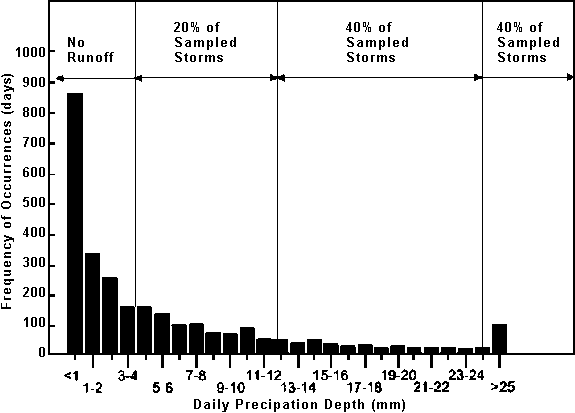
A major benefit of reviewing sample representativeness during the course of a monitoring program is that it helps to guide subsequent monitoring efforts by identifying those types of storms which to date are underrepresented in the sampling program. Figure 46 illustrates the results from a monitoring program with respect to a long-term study of precipitation volumes at the same site. The results of the program illustrated in Figure 46 are disproportionally weighted to larger storms' depths. A BMP evaluation using this data set would not be representative of the more frequent smaller storms that may have been the basis for the design of the BMP being evaluated.
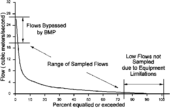
Since the relationship between rainfall and hydrologic response varies with antecedent conditions, a more accurate representation of sample representativeness can be obtained using a preexisting flow duration curve for the monitoring site. Alternatively, a similar curve can be generated using a locally available rainfall record and a hydrologic/hydraulic model of the BMP to be evaluated. The flow duration curve can also be used to permit a preliminary evaluation of the types and amounts of flows that may be missed during the course of the monitoring program (Figure 47).
Equipment Needs and Selection. The field equipment requirements for a manual or automated sampling program can be supplied by a wide range of vendors.
Manual Sampling. Manual sampling programs are initiated for several reasons including (1) a preliminary constituent screening process used to identify the occurrence and expected range of particular constituents done in the program design phase; (2) limited resources for equipment purchases and installation; (3) availability of personnel to complete the sampling; and (4) some constituents such as bacteria, oil and grease, and volatile organic compounds (VOCs) are difficult to sample for with automated equipment.
While not as critical as in the case of automated sampling, the selection of equipment to assist in manual grab sampling is also important. It is usually advisable to use a hand-held grab sampler to permit samples to be collected safely and without the risk of contamination (McCrea and Fischer, 1993).
Automated Sampling. For an automated sampling program, the minimum equipment generally needed includes both automated water samplers and stage recording devices located at the inlets and outlets of the BMP to be evaluated or at instream locations.
Water sampling equipment selected must have the capability of meeting the requirements for sample volume, and sample numbers specified in the design phase of the monitoring program. The programming capabilities of the sampler must also permit various sampling protocols (discrete, composite). Automated units can be powered from a nearby utility connection or from stand-alone battery units. If power can be supplied from a utility connection, a refrigerated sampling unit is commonly purchased. This ensures that samples are cooled and preserved immediately. Sampling units using battery power generally require the sampler to be packed with ice prior to a sampling event.
A stage or flow recorder and its sensor and a water sampler can be purchased as an integrated unit or purchased as two separate stand-alone units. Operationally, both setups are similar; however, the integrated units are generally smaller and as a result can be placed in confined spaces such as access holes. Integrated units also tend to have greater programming flexibility. A disadvantage of the integrated units is that the flow meter cannot be used separately from the water sampler. The selected sensor for stage recording will need to be sensitive at the expected range of velocities found at the sampling location.
To obtain representative flow information, a hydraulic evaluation of the flow velocities at all sampling points must normally be completed not only for sensor selection, but also for the selection of stage recording or flow metering equipment.
A decision to install a primary measuring device such as a weir or flume or to develop an in situ stage-discharge relationship must also be made in conjunction with the purchase of a stage recorder and sensor. Estimates of the expected depths and discharge rates at the proposed sampling location are required for both methods of determining discharge. Several hydraulic handbooks are available to guide the selection process for a primary measuring structure (for example, Bos, 1988). Recommendations for stage sensor selection and placement, and features of the approach section are normally dependent on the type of structure used.
Hand-held discharge measuring equipment is also required to perform checks on a primary measuring device and to develop an in situ stage-to-discharge relationship. The equipment selected must be physically capable of measuring discharge at the expected range of depths and, as mentioned earlier, flow velocities.
To further characterize the conditions under which samples have been collected, sensors to monitor parameters such as rainfall, temperature, dissolved oxygen, pH, turbidity, or conductivity can also be added to monitoring programs. At a minimum, a rainfall sensor should be considered for assistance in evaluation of BMP performance and of the sampling program's representativeness. More than 50 percent of the monitoring studies reviewed had measured both rainfall amount and intensity during the course of BMP evaluation. Most of the remaining studies did not report rainfall parameters. Continuously monitoring the changes in water temperature, dissolved oxygen concentration, pH, and turbidity is particularly important since changes in these parameters often increase the toxicity or impacts of pollutants in stormwater.
To protect automated monitoring equipment from vandalism and theft, an instrument shelter is often purchased or constructed at the sampling site. Fiberglass enclosures are generally the most commonly used and are easy to handle and install in the field.
Sediment Sampling. Several BMP designs use sedimentation or filtration processes to remove constituents from stormwater. As a consequence, these sediments and filter media become sinks for these constituents, which accumulate over time.
Evaluations of the levels to which these constituents accumulate can be indicative of the removal efficiency of a particular BMP. Their levels can also affect disposal options, as in the case of the removal of accumulated sediment from a BMP, or when filter media is removed from a filtration type BMP.
To collect samples for analyses, a small, hand-operated auger can be used to collect samples from either filter media or accumulated sediments. Additional and more detailed procedures outlining sediment sampling devices and procedures for both sediment grain size and sediment chemistry can be found in USEPA (1991) and Young et al. (1996). Standardized procedures are also available for the sampling of sediment in water flow from the United States Geological Survey (USGS, 1982).
|
Sediment Sampling
A total of eight modified Delaware sand filter (DSF) BMPs were constructed to treat stormwater runoff from a 5 ha (12.4 ac) container shipping and storage terminal yard for Alaska Marine Lines (Horner and Horner, 1995). In additional to evaluating the pollutant removal effectiveness of the BMPs, a separate analysis was made of the condition of the sediments accumulated in the setting chambers and the condition of the sand beds in the filter chambers to define potential maintenance needs. Sediment samples from the settling chambers and 25.4 mm (1 in) sand cores from the filter chambers were collected separately for analysis. Particle size distributions and pollutant concentrations in sand samples collected from two of the filters were compared with those of clean sand to assess changes that had occurred during the seven months of operation prior to sampling. Pollutant concentrations in sediment and sand were also compared.
Based on sand core analyses after seven months of operation, it is estimated that the sand filter systems will provide several years of service before needing major maintenance. Sediment samples from the settling chambers and whole sand cores from the sand chambers did not come close to violating any leachable metals criteria for designating hazardous or dangerous waste. However, the sediments exceeded total petroleum hydrocarbon (TPH) criteria under toxics control legislation and would have to be treated as hazardous waste when removed during maintenance.
|
Large Volume Sampling. Special large-volume centrifuge systems are used to recover sufficient material for the analysis of trace organic constituents such as PAHs. These systems are labor-intensive and are practical only for use in low-intensity monitoring programs. Commercially available samplers that have been used in monitoring studies include the Westphalia KDD 605 (Savile, 1980) and the Alfa Laval (Ongley and Blachford, 1982).
Field Measurements and Sampling Methods
Each type of field operation will require the development of standard operating procedures (SOPs), which document the data collection and measurement processes, or the requirements for routine maintenance on equipment such as automated samplers. SOPs cover all aspects of fieldwork relating to data quality and assurance, from the type and frequency of equipment maintenance to calibration, cleaning, and adjustment requirements. Records of equipment maintenance, malfunctions, calibrations, and adjustments need to be kept for each monitoring station. These SOPs are often based on existing published standards or procedures developed for site-specific conditions. Guidance on the development of SOPs can be found in documents such as the Guidance for the Preparation of Standard Operating Procedures (SOPs) for Quality-Related Documents (USEPA, 1995).
For standard operating procedures specific to water quality and discharge monitoring, the Handbook for Sampling and Sample Preservation of Water and Wastewater (USEPA, 1982), Water Quality Monitoring (USDA, 1993) and National Handbook of Recommended Methods for Water-Data Acquisition (USGS, 1977) can be consulted.
Training and Logistics Program
Monitoring programs are often completed by several different people over the course of months or, in some cases, years. To ensure the long-term consistency of data collection procedures, individuals involved in monitoring programs need to be systematically trained in the use of equipment, and its calibration and maintenance requirements.
The success of monitoring programs that focus primarily on the sampling of storm events relies heavily on the ability of personnel to respond in a timely manner. As a consequence, it is advisable to develop clear procedures for the deployment of sampling personnel and their alternates.
Monitoring programs can potentially generate a lot of valuable data. The data can be used for multiple purposes as monitoring efforts attempt to address BMP effectiveness at both the local and regional level. Monitoring data may be shared by various agencies to allow more informed decisions to be made about stormwater management and BMP implementation. It is necessary to have a well-structured data management system in place to host monitoring data.
The use of an ad hoc data management system prevents efficient retrieval of the data and can potentially lead to the loss of valuable data. It is important to design and develop a structured database management system (DBMS) once it has been determined what kind of data will be collected during the monitoring program. The preliminary DBMS design should ideally be completed before implementing the monitoring program. A flat-file DBMS may be sufficient to meet the needs of relatively small monitoring programs. However, DBMSs based on more sophisticated data models may be required for larger monitoring programs. Relational DBMSs are widely used in a variety of applications and have become the de facto standard for developing large-scale databases.
Database Design Considerations
A well-designed DBMS offers several advantages, including:
- Storage and rapid access capabilities for large amounts of data.
- Data revision and reuse without extensive reformatting.
- Simplified data reporting.
The database design process should include the following steps:
- Assess the purpose of the database, including data storage needs and possible queries that may need to be processed (e.g., storm characterization, continuous flow characterization, wet weather and dry weather sampling results).
- Based on the assessment of data storage and retrieval needs, divide the information into separate subjects that will be separate tables (e.g., rainfall measurements, flow measurements, wet weather sampling data and dry weather sampling data, BMP characteristics, maintenance requirements).
- Determine the various components (fields or columns) making up the information in each table (e.g., the fields in a rainfall measurements table could be: date storm started, time storm started, date storm ended, time storm ended, and total storm precipitation).
- Test and refine the preliminary design by adding a few hypothetical records and determining if the desired information can be rapidly processed and obtained from the database.
If a relational DBMS is selected for hosting the data, the third step includes establishing links between the various tables and reassessing fields and tables to ensure there will be no data redundancies. Each table in a relational database includes a field or set of fields (referred to as the primary key) that uniquely identifies individual records in the table. Relational databases use primary key fields to efficiently associate data from multiple subject tables.
Regardless of the level of database sophistication, it is advisable to include basic features for checking errors and indicating data quality in the database design. This practice assists in meeting the data quality objectives of the monitoring program and is useful in establishing procedures for data processing and reduction for analysis and reporting. Typical error checking features include measures to prevent the inadvertent entry of data outside a range of acceptable values for a particular constituent. Standard codes should be used to indicate instances when constituent concentrations fall below the analytical detection limit or when data is missing.
Separate fields should be included for flags to indicate data reliability. This occurs when data has been collected, but its representativeness is uncertain for a number of reasons. For example, some samples may be analyzed for a constituent after the maximum recommended holding time for the constituent has expired or samples may have been incorrectly preserved or stored. In other instances, trash or sediment may have accumulated or have may been trapped by the sampler intake, mounting or sampler lines, resulting in some questions about the representativeness of the samples taken. The occurrence of any of these or similar conditions will have been recorded in the field notebook for the monitoring station. While the initial decision concerning acceptability of this data will be, by necessity, the responsibility of experienced field personnel, a final decision should be made by qualified staff during data review and validation process.
Data Processing
Data processing essentially involves operations on the raw data to provide a new data set that can be directly used in analysis. For example, a common data processing operation involves replacing data generated from chemical analysis that fall below the limit of the analytical procedure by a value equal to one-half of the detection limit if the percentage of nondetects is less than about 15 percent of the total number of samples (USEPA, 1996). When the number of nondetects exceeds 15 percent of the total samples, adjustments are usually made in analysis methodology. Other examples of data processing operations include:
- Estimation of missing values (e.g., through interpolation in continuous flow measurements).
- Data reduction (e.g., the computation of event mean concentrations of constituents by storm event using data for discrete samples [see Section 4.6.1]).
- Data conversion (e.g., the conversion of stage to discharge data using a rating equation [see box]).
Monitoring data should be entered, processed, and reviewed immediately following its collection and reporting and on a periodic basis. This allows corrective action to be promptly taken should problems exist in either the data collection, data processing, or analysis procedures.
|
Development of A Rating Equation
The following steps are recommended to develop the rating equation (USDA, 1993):
- Log transform paired values of discharge (Q) and stage (H)
- Perform a linear regression of Q vs. H with Q as the dependent variable
- Obtain intercept (C), and slope (b)
- Add coefficients to the equation:
logQ = logC + b@logH
- 5. Transform equation to the form:
Q=CHb
by taking the antilog of the equation in step 4,
so that:
Q=10CHb
For example, if the intercept (C), was 0.05 and the slope (b) was 2.54, the equation would be:
Q=100.05@H2.54
or
Q=1.12@H2.54
|
The sampling design plan, data management, data collection procedures, training, and logistics considerations, and their QA/QC components are usually compiled into a quality assurance project plan (QAPP). The QAPP is normally prepared prior to beginning monitoring and distributed to all staff involved in any of the activities of the monitoring program to guide implementation of the program (see USEPA, 1994a). The QAPP specifies, in an organizational chart, the roles and responsibilities of each member of the monitoring program team from the project manager and QA/QC officer to the staff responsible for field sampling and measurement. Project management responsibilities might include overall project implementation, sample collection, and data management. Quality management responsibilities might include conducting checks of sample collection or data entry, data validation, and system audits. The QAPP also describes the tasks to be accomplished, the data quality objectives for the kinds of data to be collected, any special training or certification needed by participants in the monitoring program, and the kinds of documents and records to be prepared and how they will be maintained.
The term "quality" relates to the degree of confidence that one can have in the results obtained for a particular analysis. Quality control is a system of technical activities that measure the attributes and performance of a process, item, or service against defined standards to verify that they meet stated requirements. Quality assurance is an integrated system of management activities involving planning, quality control, quality assessment, reporting, and quality improvement to ensure that a product or service meets defined standards of quality with a stated level of confidence. QA and QC procedures are detailed in the QAPP, to address the sampling (data collection) design, what methods will be used to obtain the samples, how the samples will be handled and tracked during the project, what specific protocols and analytical methods will be used to estimate the levels of specified water quality parameters in the samples collected, what control limits or other materials will be used to check performance of the analyses (QC requirements), how any instruments or other equipment used will be inspected and calibrated, how supplies will be inspected, how nonmeasurement data will be acquired and used, and how all data generated during the monitoring program will be managed and errors in data entry and data reduction controlled (Keith, 1991).
Standard operating procedures (SOPs) are referenced in the QAPP; SOPs provide a step-by-step description of technical activities to ensure that project personnel consistently perform sampling, analysis, and data handling activities throughout the duration of the project so that data comparability is maintained. The use of standard methods of analysis for water quality parameters also permits comparability of data from different monitoring programs. Changes in equipment or measurement methods are also incorporated into the original SOPs as dated amendments.
The types of assessments to be conducted to review progress and performance (e.g., technical reviews, audits) and how nonconformance detected during the monitoring program will be addressed are also discussed in the QAPP. Finally, procedures are described for reviewing and validating the data generated, dealing with errors and uncertainties identified in the data, and determining whether the type, quantity, and quality of the data will meet the needs of the decision makers.
The QAPP is prepared during the monitoring design phase of the monitoring program to document all technical aspects of the data collection effort that will be implemented and provides the basis on which the data collection effort can be evaluated. The QAPP should be continuously refined to be consistent with changes in field and laboratory procedures. Each refinement should be documented and dated to trace modifications in the original plan.
Sample Handling and Reporting
Many monitoring programs submit water/sediment samples to an outside analytical laboratory for constituent analysis. As a result, it is important to work out the logistics and QA/QC elements of sample submission prior to collecting any samples. This normally requires establishing written data collection and chain-of-custody standards and ensuring that they are adhered to throughout the monitoring program.
"Many monitoring programs submit water/sediment samples to an outside analytical laboratory for constituent analysis. As a result, it is important to work out the logistics and QA/QC elements of sample submission prior to collecting any samples. This normally requires establishing written data collection and chain-of-custody standards and ensuring that they are adhered to throughout the monitoring program.
To ensure proper handling and preservation of water quality samples, sample bottles should be clean and appropriately labeled with an indelible marker prior to going into the field. The labels for each sample should contain information concerning the sample location or station, date and time collected, collectors name, air temperature if appropriate, and any preservative added. Methods describing recommendations for preservation, handling, and detection limits for commonly analyzed constituents can be found in Standard Methods for the Examination of Water and Wastewater (APHA, 1995).
In addition to proper handling, preservation, and storing, the effectiveness of any monitoring program depends on its quality control (QC) component. The goal of the QC program is to provide a quantitative measure of the accuracy of the collected data. This includes procedures for both the field and analytical portions of the data collection process. For some variables, QC involves calibrating instruments, such as pH and conductivity sensors, with known standards.
To ensure accuracy and precision, analyses of blanks, replicate samples, control samples, and spiked samples may all be required for QC. Field replicates are samples collected simultaneously at the identical source location and analyzed separately. This type of analysis assesses the total sample variability, both random and systematic. Laboratory replicates consist of repeated analyses of a constituent performed on the contents of a single sample. This type of test assesses the random variability or precision in the analytical analysis. Controlled samples or spiked samples determine the ability of the laboratory equipment or procedures to detect specific types of constituents at known concentrations. The procedures used by an individual laboratory are normally well documented and can be obtained upon request. It is still generally advisable, however, to arrange for a small percentage of the samples collected (e.g., 10 percent) to be submitted to a second laboratory.
|

