Roadside Revegetation: An Integrated Approach to Establishing Native Plants and Pollinator Habitat
Chapter 6 – Monitoring
Table of Contents
6.1 INTRODUCTION
The goal of roadside revegetation is to establish plant communities along roadsides and other road-related disturbances that meet project objectives.1 In practice, however, roadside revegetation projects rarely turn out exactly as planned. Therefore, regular visits to the project site to evaluate progress, and to intervene if necessary, are important parts of the revegetation process.
Monitoring is carried out for two reasons: (1) to correct, manage, and maintain the project effectively and (2) to learn what went right or wrong and apply this knowledge to future projects. Monitoring provides the answers to the following questions:
- Were revegetation goals and expectations met?
- Is native vegetation establishing appropriately or should corrective action be considered?
- Were desired future conditions (DFC) targets met?
- Are there differences in plant responses between different revegetation treatments?
- How are pollinators responding to revegetation treatments?
- Did revegetation result in a plant community capable of supporting a diverse pollinator population?
- Should the revegetation methods and techniques strategy be revised based upon monitoring data?
Answers to these questions may be obtained in a variety of ways depending on the purpose and needs of the project; however, a monitoring plan that can be applied to all revegetation projects does not exist. Instead, a monitoring plan is tailored to the objectives of each project and to the unique characteristics of the site. In developing a monitoring plan, it is important to determine the type and intensity of monitoring in advance. Simple field visits or photo point monitoring over time may provide sufficient information to determine whether objectives have been met, whereas statistically based procedures, outlined in Section 6.3, may help determine if specific targets were achieved. Regardless of the intensity of the strategy, consistency and a long-term commitment are keys to successfully implement an informative monitoring strategy.
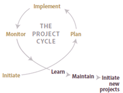 Figure 6-1 | Monitoring and the project cycle
Monitoring completes the project cycle and the results are used to guide future management and maintenance work. Monitoring can also provide insights for improving future projects.
Monitoring completes the project cycle by providing feedback regarding the success or failure of a revegetation project. This information can be used to adapt and improve other revegetation projects that are in the initiation, planning, or even implementation phases (Figure 6-1). Information collected during monitoring can help determine if corrective actions, such as adjusting seed mixes or follow-up management activities (e.g., reseeding or replanting), are appropriate. Monitoring results may also be used to improve revegetation techniques for future projects.
The monitoring phase may include the following steps:
- Determining what aspect of the project is to be monitored
- Developing a monitoring plan
- Collecting field data
- Analyzing field data
- Applying corrective measures
- Writing up findings
This chapter begins by describing monitoring plan development and moves through collecting, analyzing, and summarizing data in a monitoring report. A set of procedures are included that outline data collection for different plant, soil, and pollinator attributes.
Back to top
6.2 DEVELOPING A MONITORING PLAN
Monitoring projects often fail because the purpose, goals, and monitoring methods are not clearly defined. The development of a monitoring plan is a process that clarifies what is to be considered prior to going into the field. Since field time is very expensive, development of a monitoring plan in the office can save valuable field time and improve the quality of the data being collected. The monitoring plan does not have to be lengthy; in fact, most can be written in a single page. The plan will be most useful if it addresses the following points (after Elzinga et al 1998):
- Purpose—Outlining the reason for monitoring, goals, and criteria for success
- Intensity—Determining the scope
- Who—Identifying expertise needed
- What—Determining parameters to monitor
- When—Determining frequency
- Where—Delineating where sampling will occur
- How—Selecting the monitoring procedures for data collection and analysis
- Logistics—Defining timeline, budget, data management, and equipment
These points become the backbone of the monitoring plan.
6.2.1 OUTLINING THE REASON FOR MONITORING (PURPOSE)
A common pitfall in many monitoring projects is the lack of clearly stated objectives or reasoning behind field visits and data collection. A good monitoring project is not defined by the amount of data collected, but whether the data adequately and effectively answered whether the objectives of the revegetation project were met. Successfully answering this question is only possible when the objectives for monitoring are clearly stated. Monitoring efforts not only link back to the original project objectives, but also to the specific DFCs developed in the planning phase (Section 3.2 and Section 3.7). Objectives and DFCs set the targets (sometimes referred to as “performance standards,” “thresholds,” “success criteria,” or “indicators”) against which the project is evaluated (Clewell 2004).
A monitoring plan begins with a statement of purpose or reason for monitoring. This is often a restatement of the objectives and DFCs of the revegetation project. If the objective of a revegetation project is to improve pollinator habitat by increasing the cover and diversity of native plants, then the monitoring plan would focus specifically on those elements pertaining to species diversity and plant cover and avoid collecting extraneous data. In addition, monitoring native bees and monarch butterflies would indicate how populations of insects have responded to the resulting plant composition. Time will be saved and the value of the data will be increased by streamlining data collection to include only the information needed to answer the question of whether the project met the objectives or DFCs stated in the plan.
DFCs are often stated in quantitative language. For example, the DFCs for a cut slope three years after construction could be stated in the revegetation plan as “less than 25 percent bare soil will be exposed” and “vegetative cover will be composed of greater than 70 percent native species.” These DFCs are very specific and can be used as target values, or thresholds, for determining whether the project was successful. Monitoring methods, or procedures, are developed specifically around each of these DFC targets. When monitoring is approached in this manner, only the information needed to determine whether targets were met is collected. Expensive, superfluous data collection is avoided because the DFC targets are clearly defined. The monitoring plan defines how this information will be measured and evaluated. After field data is collected, the DFC target values can be used to evaluate success or failure and whether corrective action is needed.
6.2.2 DETERMINING THE INTENSITY (INTENSITY)
The scope of data collection will depend on the size and importance of a revegetation project. Not all revegetation projects will involve the same intensity of monitoring to meet project goals. Some portions of the revegetation project might entail only a field review and a series of photographs, while other areas within the project will involve a statistically designed monitoring procedure. At a minimum, most projects call for annual visits and recorded observations or qualitative assessments.
Portions of revegetation projects may benefit from statistically based monitoring procedures. For example, if a project has a water quality goal for sediment control that road sections near a high-value fishery have no greater than 20 percent bare soil for sediment control the first year after construction, the importance of this project to fisheries and water quality would underscore the importance of high confidence in the accuracy of the data. This could involve more intensive data collection and statistical analysis to ensure a higher level of certainty. Alternatively, road sections that do not affect the stream system may not involve the same level of effort. In such cases, qualitative assessments, such as photo point monitoring, may suffice (Section 6.5). In general, the scope of monitoring reflects the importance of the revegetation objective, ecological sensitivity of the project area, and budgetary constraints. The levels of monitoring intensities include the following:
- Low—Site visits, field notes, photographs
- Moderate—Photo point monitoring
- High—Statistically based data collection and analysis
6.2.3 IDENTIFYING THE NEEDED EXPERTISE (WHO)
For efficiency and safety, a minimum team of two people is recommended for revegetation monitoring. The team is typically composed of the designer, or someone familiar with the revegetation project, and a person trained in plant identification. If parameters, such as soil characteristics are being monitored, then a person with soils background would also be involved, or if pollinator surveys are being conducted, then the team would have a person knowledgeable in identifying pollinators.
It is important to have one person be responsible for all monitoring activities. This person develops and implements the monitoring plan, conducts data collection and analyses, and completes the final monitoring report. It is advantageous that the project designer or personnel who planned and implemented the revegetation project be involved with data collection and even be the person that oversees the monitoring activities. Monitoring is often delegated to others with less knowledge of the project, but a great opportunity for learning is lost when this occurs. Monitoring is the feedback loop for the designer and implementer to make improvements on the next project.
6.2.4 DETERMINING MONITORING FREQUENCY (WHEN)
Specifying the timing of data collection in terms of years following project completion is important in determining if DFC targets have been met. Monitoring that occurs within a year after project completion is conducted to assess whether some areas need to be reseeded or replanted, and to determine efficacy of erosion-control devices (fabric, wattles, mulch, etc.). This low intensity monitoring is often conducted through site visits during which ocular estimates are made. Assessing the long-term success of a project is done three or more years after revegetation treatments have been completed. Some portions of a revegetation project may warrant more than one sampling visit. For example, a planting contract with a DFC of 400 live trees after the first year of planting and 300 trees alive after three years would be monitored the first and third years after planting.
Specifying the month or season when a project is monitored is also important. If the identification of individual plant species is the monitoring goal, monitoring is scheduled during the appropriate phenological window for plant identification. The bloom period is also the time when pollinators are sampled since this is when their populations are at their greatest. If outplanted stock is to be measured for survival or growth, the appropriate time to monitor is after seedlings have become established, which is typically 6 months to a year after planting. For climates with extended dry periods, common to the western United States, this monitoring is typically conducted in the fall. Alternatively, the collection of soil cover data for erosion control is done prior to intense rainstorm periods, which in New Mexico, Arizona, Colorado, Utah, and Texas is in the summer; for Gulf States, it is in the late summer and fall; and for the western United States, it is in fall and winter.
Bee populations vary seasonally and annually. For this reason, it is important for pollinator monitoring to sample a project more than once. For example, it may take several years for a newly seeded area to become established before there is an increase in pollinators. On these sites, monitoring pollinators the first year after seeding may not yield as much useful data as the second and third year, which may be the best years for monitoring. Pollinator surveys are best conducted when plants are flowering, which may warrant two or three surveys a year, especially if there is a variety of flowering species with different bloom times. Depending on the region, this can be in late spring/early summer, mid-summer, and late summer.
6.2.5 DELINEATING SAMPLING LOCATIONS (WHERE)
The sampling unit is the area in which a specific monitoring procedure will be used. Revegetation projects may be monitored as one sampling unit or several. A way to determine the locations of the sampling units is to revisit the revegetation unit map developed for the revegetation plan (Section 3.4). If the project is large or complex, some or all of the revegetation units may be treated as separate sampling units. Referring to the purpose for monitoring at the beginning of the monitoring plan helps identify the most important areas to monitor. For example, if the purpose for monitoring is to determine whether water quality objectives were met, only the areas adjacent to drainages and waterways would be delineated for high intensity monitoring, leaving the remainder of the project for low or moderate intensity monitoring. If the monitoring objective is to determine how well native plant species established, then setting up a sampling unit that would cover the entire revegetation project area may be appropriate. Comparing changes in plant or pollinator populations may benefit from locating and monitoring a nearby reference site.
6.2.6 DETERMINING PARAMETERS TO BE MONITORED (WHAT)
Clearly stating which data are essential to collect can increase the quality of the monitoring data and minimize field time. Referring to the reason for monitoring, outlined at the beginning of the monitoring plan, helps narrow the parameters for data collection. These parameters are discussed in detail in Section 6.3.
6.2.7 SELECTING MONITORING PROCEDURES (HOW)
There are many vegetation and pollinator population monitoring methods, protocols, and procedures from which to select. Using an established set of monitoring procedures, tailored to the monitoring objectives, is important because they can save time and increase the quality of the data collected. The procedures outlined in this chapter were developed specifically for roadsides and road-related disturbances. A monitoring procedure, as defined in this report, provides information for conducting monitoring. These procedures are used for moderate and high intensity monitoring. Qualitative procedures, such as photo point monitoring, are used for moderate intensity monitoring. Statistically based procedures have been developed for high intensity monitoring.
For high intensity vegetation and pollinator monitoring, there are three sets of statistically based monitoring procedures that are used together. In the development of a monitoring plan, one procedure from each of the three procedure groups is selected for each sampling unit. These are discussed in Section 6.3
6.2.8 LOGISTICS
The monitoring plan also includes a timeline that shows the periods and completion dates for field monitoring, data analysis, and the monitoring report. Included in this section are the specialists involved in monitoring, their expertise, and the estimated time involved. A budget can be developed from this information. Finally, a list of equipment can be attached to the monitoring plan.
Back to top
6.3 PLANT AND SOIL MONITORING PROCEDURES
This section describes how to develop and implement a set of statistically based monitoring procedures specific to the revegetation project. It outlines methods to record, summarize, and analyze data. Monitoring personnel can obtain spreadsheets, which include field data forms and analysis spreadsheets for each procedure, from the Native Revegetation Resource Library. To obtain a list of Excel monitoring procedure workbooks referenced in this chapter, type “xls” in the Search field.
The following three questions are answered to develop a procedure for soil and plant monitoring for each sampling unit:
- What is the shape of the sampling unit?
- What are the monitoring objectives?
- What is being monitored?
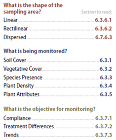 Figure 6-2 | Quick guide to high intensity monitoring procedures
For statistically based monitoring of plant and soil attributes, select a procedure that best answers each of these questions.
The answer to these questions will lead the designer to draw from different sections of this chapter. Take, for example, a road cut that is being monitored to determine if soil cover targets conformed to the Storm Water Pollution Protection Plan. Using Figure 6-2, the Linear sampling area procedure would be used because the road cut is long and narrow. Since the objective is to determine if soil cover targets were met, the Compliance and the Soil Cover procedures would be used.
Sampling Unit Shape
The shape of the sampling area is important for determining how transects and quadrats are laid out in a sampling unit. For roadside monitoring, there are three main shape categories to choose from, each with a corresponding procedure:
- Linear—This shape is long and narrow and is used to monitor cut slopes, fill slopes, and abandoned roads (Section 6.3.6)
- Rectilinear—These sampling areas are typical of staging areas, material stock piles, or large wide areas associated with road construction (Section 6.3.6)
- Dispersed—A series of discrete areas that include planting islands and planting pockets (Section 3.8.2, Section 5.2.8, Section 6.3.6)
Parameters to be Monitored
Parameters for monitoring revegetation projects may include the following, depending on monitoring objectives:
- Soil cover—The amount of exposed bare ground is used to determine if treatments produced adequate soil cover for erosion control (Section 6.3.1)
- Species cover—Used to determine the percentage of aerial or basal cover occupied by individuals or groups of species to quantify species prominence (Section 6.3.2)
- Species presence—Used to assess what species are on the site, how well species in a seed mix became established, or whether noxious, invasive, or undesirable species are present (Section 6.3.3)
- Plant density—Used to assess how many seedlings or cuttings became established after outplanting or how much mortality has occurred (Section 6.3.4)
- Plant attributes—Used to determine growth rates of outplanted seedlings or cuttings (Section 6.3.5)
- Pollinator abundance—Used to assess quantities of honey bees, native bees, and other pollinators (Section 6.4)
Monitoring Objectives
Monitoring objectives also guide how data are collected and statistically analyzed. Procedures have been developed for three basic types of monitoring objectives (Section 6.3.7):
- Compliance—This is often the main purpose for monitoring. It is used to determine if project objectives were met or simply to summarize monitoring data
- Treatment differences—This monitoring objective examines the differences between revegetation treatments or revegetation areas. It is useful to evaluate the effects of different revegetation treatments (seed mixes, fertilizers, soil amendments etc.) on plant establishment
- Trends—This objective evaluates changes in the revegetated plant community in the disturbed area over time. It is used when it is important to understand how plant communities evolve and change
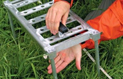 Figure 6-3 | Fixed frame for transect sampling
A fixed frame can be adapted to allow for the positioning of a laser pointer at 20 points in the frame. Soil cover or plant cover attributes are recorded at each laser point. The frame in this example is 8 inches by 20 inches, with 2-inch spacing within rows and 4-inch spacing between rows. The laser is a Class IIIa red laser diode module that produces a 1-mm dot.
Photo credit: David Steinfeld
6.3.1 SOIL COVER
Reestablishing a soil cover on disturbed sites is important for erosion control. The following soil cover procedures can be used to determine the amount and type of cover existing on the soil surface after slopes have been constructed. The quadrat is the unit of area monitored for soil cover. Exact measurements are based on recording the surface soil condition at data points within each quadrat. Quadrats can be read in the field using a fixed frame or read later in the office from digital photographs of the quadrat taken in the field (Section 6.3.1).
Sampling Soil Cover Using a Fixed Frame
Soil cover is quantified at each quadrat based on readings from a 20-point fixed frame. This method is a point intercept method of estimating cover in a defined area (quadrat). Several types of frames have been developed. The most useful frames are lightweight, portable, and stable. One frame that meets these criteria uses a laser pointer to identify data points. The frame shown in Figure 6-3 has 20 slots to position a laser pointer. During monitoring, the laser pointer is moved to each of the 20 slots. Soil cover attributes are recorded where the laser hits the ground surface.
The fixed frame is located along the tape in a consistent manner throughout the sampling of a unit (Figure 6-4). For example, the frame might be placed on the right side of the tape with the lower corner of the frame at the predetermined distance on the tape. This procedure would be applied consistently across the entire sampling unit. The legs of the frame are positioned so that the surface of the frame is on the same plane as the ground surface.
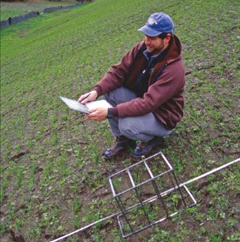 Figure 6-4 | Fixed frame for measuring soil cover
A fixed frame for measuring soil cover is placed at predetermined distances on a transect.
Photo credit: David Steinfeld
Each data point is characterized from a set of predetermined label descriptors that include, but are not limited to, the following:
- Soil
- Gravel (2 mm to 3 inches)
- Rock (>3 inches)
- Applied mulch
- Live vegetation (grasses, forbs, lichens, mosses)
- Dead vegetation
Ideally, only cover in contact with the soil surface is considered effective ground cover for erosion control purposes; however, differentiating between plant leaves and stems that are in direct contact with the soil as opposed to simply in close proximity to the soil surface can be difficult and is not always feasible. In this procedure, the assumption is that if live or dead vegetation is within 1 inch of the soil surface, it is recorded as soil cover.
Vegetation often blocks the view of the soil surface and is therefore removed prior to data collection. When this is the case, the quadrat is clipped of standing vegetation (dead or alive) at a 1-inch height above the ground surface prior to taking the readings. The clipped vegetation is removed from the plot before the reading is made.
Data can be recorded on a field computer or field recording sheets. Field recording sheets bypass the need for electronic equipment in the field; however, data is entered into a spreadsheet at a later time for analysis. An Excel workbook with field entered forms and a data analysis package (see Figure 6-5) is available for this procedure in the Native Revegetation Resource Library.
Sampling Soil Cover using Digital Photographs and the Cover Monitoring Assistant (CMA) Program
For the Designer
Find this and many other fillable spreadsheets in the Native Revegetation Resource Library by typing “xls” into the search field.
Digital cameras are being used more frequently for monitoring plants and animal life. This technology allows the data recorder to spend most of the field time laying out transects and taking photographs of quadrats rather than collecting data, thereby reducing field time significantly. With recent developments in photo-imaging software, photographs can be assessed quickly in the office. Because these are permanently stored records, digital photographs have several advantages: photographs can be reviewed during the “off” season or “down time”; they are historical records that can be referenced years later; and they can be reviewed by supervisors for quality control. In addition, taking digital photographs of ground cover can be accomplished by one person, not two as is often used for fixed-frame monitoring. On steeper slopes, taking photographs to record quadrats is quicker and easier than reading attributes from a fixed frame.
Sampling by camera entails the same statistical design and plot layout as the fixed-frame method. The photograph is taken within a quadrat frame with 11-inch by 14-inch dimensions, covering approximately 1 square foot. In the office, digital photographs are catalogued electronically and a 20-point overlay is placed on the image that identifies the data points to be described (Figure 6-6). The data points are described in the same manner as for the fixed-frame method.
The FHWA and the U.S. Forest Service have developed a computer program to evaluate digital photographs called Cover Monitoring Assistant (CMA). This program configures each digital photograph taken at a quadrat so it is easy to evaluate in the office. It randomly places 20 points on the photograph and navigates the user to each point where the soil cover attribute is recorded. The data for each photograph is summarized in spreadsheets for statistical analysis. The CMA program has reduced field time and increased data quality significantly. The CMA program information and the User’s Guide are available in the Native Revegetation Resource Library.
6.3.2 SPECIES COVER
The species cover procedure is used to assess the above-ground abundance of plant species. This method is a point intercept method of estimating cover in a defined area (quadrat). This procedure can be used when DFC targets state that a certain percentage of vegetative cover be composed of native species. For example, a DFC target from the revegetation plan states that over 50 percent of the vegetative cover existing on the site two years after construction will be composed of native forb species for pollinator habitat and that this cover will consist of species that were in the seed mix. Monitoring vegetative cover with this procedure will determine whether this goal was achieved.
Another advantage of evaluating species cover is the elucidation of patterns of co-occurrences. Weedy species can occur in isolated patches, but often co-occur with other weeds and even among native species. Understanding these distributional patterns and the density of the species assemblages, as they change and develop with the project site, can help the designer select the most effective treatment methods, reduce redundant treatment costs, and prevent damage to the existing native plant community.
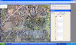 Figure 6-6 | The CMA program reduces field time
Using the CMA program for determining soil cover and/or species cover, each quadrat photo is overlain with a 20-point grid that is randomly placed. Beginning with the first point, the user determines that point lands on a rock and that cover code is entered. The program moves the recorder to the next point until all 20 points are entered. The cover codes are decided by the recorder. In this example, plant cover was detected along with soil, mulch, and rock cover codes. In this case, three plant species were identified (shown as the abbreviations BRCA, ELEL, and FEID) as discussed in Section 6.3.2.
Photo credit: David Steinfeld
Because grass and forb cover changes during the growing season, the timing of species cover monitoring is important. It is ideal to monitor when most plants are flowering, typically mid-May through July for the western United States and July through August for the upper mid-western and eastern states. Bloom periods for forb species also coincide with the optimum period for monitoring pollinator species, so monitoring for species cover and pollinators can be done during the same field visit (Section 6.4).
This sampling procedure typically benefits from a botanists’ knowledge to identify species and another person to help lay out the plots and record data. Sampling can be done either with a fixed frame or digital photographs using the CMA program.
Sampling Species Cover Using a Fixed Frame
Using the fixed frame discussed in Section 6.3.1, 20 points are identified in the quadrat frame. At each point, the species is identified and recorded in a ruggedized computer or on a field recording sheet. Species cover is quantified at each quadrat based on readings from a 20-point fixed frame. At each point, the species is recorded on a spreadsheet which is available on the Native Revegetation Resource Library.
Sampling Species Cover & Floral Density using Digital Photographs and CMA
The CMA program, discussed in Section 6.3.1, can also be used for determining species cover when plant species are easy to identify from digital photographs. These include species that are in bloom or with seed heads. Species of interest, such as those species used in a seed mix, may be the only species to identify for the analysis, requiring the recorder to know the appearance of just a few species. It may also be helpful to take a range of photographs of each species of interest for later reference when photographs are being analyzed. As with using CMA for determining soil cover, a 20-point grid is placed on each digital photograph and species cover points are evaluated (Figure 6-6).
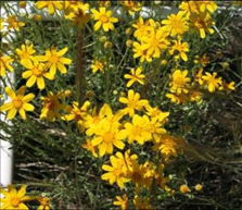 Figure 6-7 | Floral density can be determined using CMA
Floral density can be determined by counting the number of flowers for each species of interest in a quadrat, then evaluated. In this photograph, Oregon sunshine (
Eriophyllum lanatum) is the main species that is counted.
Photo credit: David Steinfeld
Floral density can be quantified using the CMA program for describing the quality of pollinator foraging habitat while photographs are evaluated for species cover. In this analysis, the number of flowers of each species of interest are counted within the quadrat frame of each photograph (Figure 6-7). A spreadsheet for this procedure is available in the Native Revegetation Resource Library.
6.3.3 SPECIES PRESENCE
The Species Presence procedure is an alternative to the Species Cover method of determining whether species are present on the site. While this method still necessitates a person knowledgeable in plant identification in the field, it takes far less time per quadrat because only the presence of a species is recorded. In this method, a fixed frame is placed on the surface of the soil at each quadrat location and the presence or absence a “species of interest” is recorded. Depending on the specific project’s success criteria, only species of interest are recorded. Species of interest may include those species that have been seeded, important pollinator supporting species, and undesirable non-native plants. If ecological restoration is a project objective, then all species may be identified.
The size of the fixed frame is based on several factors, such as the growth pattern of the species of interest and the frequency that the species is present on the site. Large frames are not necessary for most grass and forb plant communities. The 1-square-foot frame used for the Soil Cover and Species Cover procedures may suffice (the tall grass prairie systems may be an exception, requiring larger frames). Larger native woody species and undesired weedy species are often measured in quadrats with an area of 1 square meter. This size of quadrat can accommodate the patchy distribution that weedy species frequently display and, when extrapolated, can create a fair representation of the plant species’ frequency across the project site. An Excel workbook with field forms and a data analysis package is available in the Native Revegetation Resource Library for this procedure.
6.3.4 PLANT DENSITY
Trees, shrubs, and wetland plants are typically established from containerized plants grown in nurseries and planted at a specified density depending on the project objectives. Monitoring the density of live plants after they are planted is important to determine how many plants have survived and whether the site will need to be replanted.
The quadrat in this procedure is a circular plot with a specified radius. For trees and shrubs, it is recommended a 1/100 acre plot be used, which has an 11.7-foot radius and covers 436 ft2. A staff is placed at the plot center and a tape or rope is stretched 11.7 feet. While one person holds the staff, the other walks the circumference of the plot and counts the number of plants of each species within the quadrat. This information is recorded on a spreadsheet, such as that shown in the form available in the Native Revegetation Resource Library. This spreadsheet summarizes the total plants per acre and the number of plants per acre by species. Note: for linear sampling areas, only one quadrat is placed randomly within the transect.
Plant density monitoring that is used to determine survival rates are called survival surveys and these are usually conducted six months to a year after planting. If the site is planted in fall or spring and monitoring occurs the following fall, the results are referred to as the “first year survival.” Plant density monitoring thereafter is referred to as the years after planting (e.g., third year sampling is “third year survival”).
6.3.5 PLANT ATTRIBUTES
This procedure can be used to assess plant growth responses to determine how well plants are growing or whether DFC targets pertaining to growth targets were met. Typically, only sensitive areas, such as visual corridors or wetlands, have stated growth targets. This procedure might have limited applicability to most revegetation projects.
Any part of a plant can be measured for growth, and the selection of an attribute is dependent on the species being sampled. Common attributes include the following:
- Total height—trees and most shrubs
- Last season’s leader length—most trees
- Stem diameter—shrubs and trees
- Crown cover—shrubs, forbs, and grasses
Total height is typically measured from the ground surface to the top of the bud. If the plant has several leaders (or tops), the most dominant leader is used for measurement. Last season’s leader growth can be observed in most tree species. For conifers, leader growth is measured from the last whorl of branches to the base of the bud. Comparing leader growth from year to year can indicate whether plants are healthy and actively growing.
Stem diameter is also used to measure trees and shrubs. In this method, the basal portion of the plant is measured with calipers at the ground surface. Another attribute is crown cover, which is more conducive to spreading plants, such as shrubs. A large frame with grids or points is placed over the plant to obtain an aerial coverage.
Attributes for shrub and tree species uses the sampling layout and design described for plant density (Section 6.3.4) and focuses only on those species of interest that have been identified in the revegetation plan. If there are many plants of a species of interest in a quadrat, only five plants are measured. An unbiased way to select which plants of each species to monitor is to sample those plants closest to the plot center. If there are not enough plants in the quadrat to sample, then the nearest plants outside of the quadrat are sampled. The measurement for each plant is recorded on a field data sheet, available in the Native Revegetation Resource Library. Note: for linear sampling areas, only one quadrat is placed randomly within the transect.
6.3.6 SAMPLING UNIT DESIGN
The shape of the sampling unit determines how quadrats are laid out. Procedures have been developed for linear sampling areas, such as long roadsides; rectilinear sampling areas for rectangular-shaped areas such as restored borrow areas; and dispersed sampling areas, which are revegetation areas that are in patches or clumps. These three sampling designs are described below, as well as how to calculate the minimum number of quadrats to obtain an accurate representation of the sampling unit.
Linear Areas
Linear areas, such as cut slopes, fill slopes, and abandoned roads, are sampled from equally spaced transects placed along the entire length of the sampling unit. Each transect has varying numbers of quadrats, depending on the length of the transect. When the sampling unit is uniform in width, each transect will have an approximately equal number of quadrats; when the width of the revegetation unit is variable, there will be an unequal number of quadrats per transect. In either case, each transect is treated as the primary experimental unit instead of the quadrat (the primary experimental unit in this report is either the transect, quadrat, or dispersed area and is the unit for which statistical analysis is conducted).
Figure 6-8 shows a typical sampling design for a linear area. In this example, the sampling unit included only those portions of the cut slope that were seeded; it did not include road shoulders or the ditch line. For statistical analysis, the number of transects (n) to collect was estimated to be 20 based on pre-monitoring data. Spacing the 20 transects equally along the sampling unit was calculated by dividing the total length of the sampling unit by the number of transects to obtain the distance between transects (3,100/20 = 155 feet). Locating the first transect is done in an unbiased way by generating a random number between 1 and 155. A random numbers table is available in the Native Revegetation Resource Library.
Transects are laid out by establishing a line, typically a measuring tape, perpendicular to the edge of the road. The transect begins at the edge of the road beyond the ditch line and where seeding or other treatments were conducted. Each transect contains a series of quadrats spaced as follows:
- <20 foot transect length—For transects where lengths are less than 20 feet, two quadrats are placed. Two random numbers are generated between the numbers 1 and 19. These numbers indicate the location of each transect.
- >20foot and <100 foot transect lengths—For transects where lengths are between 20 and 100 feet, quadrats are placed at 10-foot intervals. The distance to the first quadrat is based on a random number between 1 and 10 feet.
- >100 foot transect lengths—Long transects have 20 feet between quadrats. The distance to the first quadrat is based on a random number between 1 and 20 feet.
When sampling units are more elliptical or rectangular in shape, or composed of several large irregular polygons, the sampling design is based on a rectangular grid of quadrats systematically located with a random starting point. Figure 6-9 illustrates an example of such a sampling design. Notice that this design is different from the linear sampling design in that there are no transects. The quadrat in this sampling design is the primary experimental unit, not the transect.
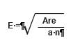
To determine the grid spacing (E) for the quadrat locations, the area of the sampling unit is calculated from maps, and the number of quadrats to be sampled (n) is determined from pre-monitoring data. The following equation gives the length of each side of a square grid (E):

For example, the sampling unit in Figure 6-9 covers 4,262 ft2 and it has been determined from pre-monitoring data that approximately 20 quadrats are necessary to attain the statistical sampling requirements for this sampling unit. The equation indicates that each side (E) of the grid is 14.6 feet:
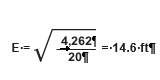
A starting point of the grid is arbitrarily located in any corner of the study area. To avoid biasing the placement of the quadrats, the corner of the grid is shifted by assigning random numbers to the x and the y coordinates, as shown in Figure 6-9. This is called a systematic design with a random start. It provides equal likelihood that any point in the study area is included in the sample unless there are obvious systematic patterns in the site, such a planting rows. In this example, the random number shifts were 11 feet in the horizontal direction and 4 feet in the vertical direction.
The monitoring team locates the random starting point in the field and measures 39.8 feet (10.6 + 14.6 + 14.6 = 39.8) north to the first quadrat. From that quadrat, they measure 14.6 feet north to the second quadrat. After they collect data from the last quadrat in that line, they travel east 14.6 feet to locate the next plot. This system of sampling continues in this fashion until the entire area has been sampled.
Dispersed Areas
When sampling units occur as small, distinct areas, a two-stage sampling design is recommended. The first stage is to determine which dispersed areas to sample, and the second stage is to determine how to sample within each selected area. For the first sampling stage, it is suggested that a minimum of 20 dispersed areas be monitored within each revegetation unit. If there are 20 dispersed areas or fewer, then all dispersed areas are sampled. If there are more than 20 areas, then sampling is conducted with one of two sampling designs. For dispersed areas that are mapped, the systematic sampling design is used. If the dispersed areas are small or are not mapped, then a grid sampling design is used. Both sampling designs are described in more detail below. These areas include planting islands and planting pockets. In most cases, the grid sampling method is recommended.
Systematic Sampling of Dispersed Areas
First Stage
The systematic sampling method of dispersed areas assumes that the dispersed areas have been mapped. The dispersed area in this method is the experimental unit. In this approach, the dispersed areas are numbered sequentially by progressing from one dispersed area to the next closest dispersed area. Determination of the number (n) of dispersed areas to sample is presented in Section 6.3.6 (see Sample Size Determination). Odd or even-numbered dispersed areas are selected based on a random number using the RANDBETWEEN function. For example, if there were 40 dispersed areas (N) but only 20 dispersed areas needed to be sampled (n), then 50 percent of the dispersed areas would be sampled (n/N). A random number using RANDBETWEEN (1, 2) is used. If the function returns a “1,” the odd-numbered dispersed areas are selected; if 2, then the even numbered areas are selected. Figure 6-10 provides a schematic depiction of such a design.
Second Stage
Once the dispersed areas have been selected, the layout of quadrats within each dispersed area is determined. A grid-based sampling design is used. To determine the grid spacing (E) for the quadrat locations, determine whether the size of the dispersed area is >1,600 ft2 or <1,600 ft2 (1,600 ft2 is a 40-by-40-foot area). Depending on the sample size, the number of quadrats will be as follows:
- Less than 1,600 feet—four quadrats
- More than 1,600 feet—eight quadrats
Using the following equation, the grid sides (E) are determined where n = 4 or 8 (depending on the size of the dispersed area) and the area is the estimated size of the dispersed area.
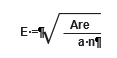
This calculation is made for each dispersed area. To avoid biasing the placement of quadrats, a predetermined starting point is made (e.g., the northwest corner of each dispersed area). Random x and y coordinates are generated for each dispersed area that is within the predetermined length of the square grid (E). The corner of the grid is placed at this point and oriented north. The location of the first quadrat is x and y feet from the starting point, as shown in Figure 6-10.
For the plant density and plant attribute procedures, only one quadrat is randomly located within each dispersed sampling area. The location is determined by assigning the RANDBETWEEN random number function to the number of quadrats determined for the dispersed area. The random number that is generated is the quadrat selected for sampling.
Grid Sampling of Dispersed Areas
First Stage
A grid sampling design is used on projects where dispersed areas have not been mapped and there are more than 30 areas. This sampling design is used on projects where dispersed areas are numerous and the sizes of the areas are small. In this sampling design, a grid is placed over the revegetation unit, as shown in Figure 6-11, and the dispersed area nearest to a grid crossing is selected for monitoring. One quadrat is randomly placed in each dispersed area and this becomes the experimental unit.
Determining the grid cell dimensions (E) is accomplished by using the following equation:
The grid is laid out in an unbiased manner by locating a starting point just outside the revegetation unit and assigning random numbers as offsets for the x and y coordinates. The corner of the grid is placed at the x and y offset point and oriented north. At each grid crossing, the closest dispersed area is selected for monitoring. If there are no dispersed areas found within half the distance between grid centers ( E / 2 ), then the monitoring team moves on to the next grid center.
Second Stage
Since the dispersed areas are small (e.g., planting pockets, planting islands, benches), all measurements for seedling density and seedling attributes may be sampled within each dispersed area. For other procedures, such as soil cover, species cover, or species presence procedures, one quadrat is located randomly in the dispersed area.
Sample Size Determination
This section covers how to take pilot data to determine the number of experimental units (transects or quadrats) needed to statistically monitor a sampling unit. It is important to note that an alternative to taking pilot data is to simply to sample a minimum of 20 primary experimental units per sampling unit. For example, for a linear sampling area, 20 transects are laid out; for rectilinear areas—20 quadrats; and for a dispersed area sampling design—20 dispersed areas). Twenty primary experimental units will provide adequate data to accurately estimate means and confidence limits and to understand the uncertainty (i.e., width of confidence intervals). The risk is that, in some cases, the intervals may be too wide to provide meaningful estimates, which means that more samples would be needed, requiring revisiting of the sampling unit. Generally, if data are moderately variable and symmetrically distributed, 20 experimental units will often be adequate (personal communication: John Kern, Kern Statistical Services Inc., February 10, 2017). The following section is intended for projects where a more exact sample size, using pilot data, is desired to achieve the precision requirements of the monitoring plan.
Sample size determination methods are tailored to the monitoring objectives and sampling area design. This section outlines four sampling methods: (1) comparing means with DFC target for linear area sampling design, (2) comparing means with DFC targets for rectilinear sampling area design, (3) comparing means with DFC target for dispersed areas, and (4) determining sample size for comparing treatment areas.
Comparing Means with DFC Targets—Linear Sample Size Determination
To calculate the minimum sample size for linear sampling areas, the expected sample mean and the range in values are approximated. A visual estimate of the mean and the range of values may be adequate. For more precise estimates, four transects are sampled in the field to establish estimates of the mean and range of values.
The following is a quick method to determine the number of transects to sample based on pre-monitoring data collection:
- Driving the entire revegetation unit and noting extremes in vegetation
- Finding four areas that represent the extremes and laying out a transect in each area
- Randomly placing two quadrats within each transect to collect data on the attribute of interest (e.g., percent ground cover)
- For each transect, averaging the quadrat values (four averages)
- Calculating the average of the four transect averages and the range (difference between highest and lowest values of the four averages)
- Applying the range and the average to the following equation to obtain the minimum number of transects needed to monitor the revegetation unit (equation based on a sample size of 20 percent of the true population value with 90 percent confidence):
n = (0.838 * Range) 2 / (0.2 * x )2
The number of transects (n) obtained from this quick assessment is used to determine the layout of the monitoring design, as described in Section 6.3.5.
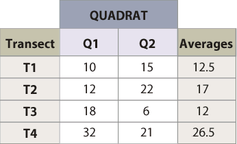
Estimated Mean = 17
Range (26.5 - 12.5) = 14.5
n = (0.838 * 14.5)2 / (0.2 * 17.0) = 12.8 transects
Figure 6-12 | Determining the number of transects using pilot data Example of how to calculate the number of transects needed, based on the pre-monitoring data set.
Example: Suppose that monitoring is to be conducted along a road cut to determine the percentage of soil cover. The monitoring objective is to estimate mean percent cover to within 20 percent of the true population value with 90 percent confidence. Four transects that represent a range in conditions are laid out within the revegetation unit. These transects do not need to be located randomly but rather can be sited to capture the range of values observed in the sampling unit. It is better to over-estimate the range of values, as this will tend to result in a conservative estimate of the sample size. The data set and equation are shown in Figure 6-12.
Using the equation presented above, an estimated 13 transects were calculated for a minimum sample size
Comparing Means with DFC Targets—Rectilinear Sample Size Determination
When a grid of quadrats is to be implemented (Section 6.3.6), the sample size calculations use quadrat measurements as opposed to the transect averages that were used in linear sampling areas. The steps involved in calculating the number (n) of quadrats are as follows:
- Visiting the entire revegetation unit and noting extremes in revegetation
- Finding four areas that represent the extremes and laying out a transect in each area
- Randomly placing two to three quadrats within each transect to collect data on the variable of interest (e.g., percent ground cover)
- Averaging the quadrat values (eight quadrat values to average)
- Calculating the range of all eight samples (difference between highest and lowest values)
- Applying the range and the average to the following equation to obtain the minimum number (n) of transects needed to monitor the revegetation unit:
n = (0.838 * Range)2 / (0.2 * x )2
Example: Using the data from the previous example (Figure 6-12), the eight quadrats would be averaged (instead of four transect averages being averaged). While the mean in this example remains 17, the range has spread to 26 (maximum 32 minus the minimum 6). The number of quadrats to sample would be 41:
n = (0.838 * 26)2 / (0.2 * 17.0 )2 = 41.126
Comparing Means with DFC Targets—Dispersed Area Sample Size Determination
Systematic Sampling Method: The systematic sampling method is used when the dispersed areas are mapped (see Systematic Sampling of Dispersed Areas). The primary experimental unit in this design is the dispersed area. The number of quadrats to sample is estimated by following these steps:
- Finding four dispersed areas that represent the extremes of the attribute of interest
- Randomly placing two quadrats within each dispersed area to collect data on the attribute of interest (e.g., percent ground cover)
- For each dispersed area, calculating the average of the four dispersed areas’ averages and the range
- Applying the range and the average to the following equation to obtain the minimum number of dispersed areas needed to monitor in a revegetation unit (equation based on a sample size of 20 percent of the true population value with 90 percent confidence):
n = (0.838 * Range)2 / (0.2 * x )2
An example of the data set and equation are shown in Figure 6-12. Note: substitute “dispersed area” for “transect” in the first column heading.
Grid Sampling Method: The grid sampling method is used for revegetation units that have small dispersed areas that have not been mapped (see Grid Sampling of Dispersed Areas). Since only one quadrat is in a dispersed area, the quadrat becomes the primary experimental unit. The number of quadrats to sample is estimated by following these steps:
- Visiting a range of dispersed areas and selecting eight dispersed areas that represent extremes of the attribute of interest
- Randomly placing one quadrat in each dispersed area and collecting data on the attribute of interest (e.g., percent ground cover)
- Calculating the average and range in values
- Applying the range and the average to the following equation to obtain the minimum number (n) of dispersed areas to sample:
n = (0.838 * Range)2 / (0.2 * x )2
Example: Using the data from the previous example (Figure 6-12), the eight quadrats would be averaged (instead of four transect averages being averaged). While the mean in this example remains 17, the range has spread to 26 (maximum 32 minus the minimum 6). The number of quadrats to sample would be 41:
n = (0.838 * Range)2 / (0.2 * x )2
Comparing Means among Treatment Groups—Sample Size Determination
When determining the sample size for comparing treatment differences (Section 6.3.7), it is not necessary to differentiate between linear, rectilinear, or dispersed sampling area designs. Sample size determinations follow these steps:
- Reviewing each treatment area to be compared. These can be different revegetation units or different types of revegetation treatments.
- From each treatment area, collecting data from two transects with each transect consisting of two quadrats (total of four transects) that represent a range of extremes.
- Determining the range between the low and high quadrat values.
- Determining delta (also represented by ∆). Delta defines the level of significance that is needed for monitoring, or the meaningful difference in measurement output. For example, calculating bare soil at 1 percent difference in means would be unimportant, that is, the difference between 8 and 9 percent bare soil is too fine a distinction to make. A 5 percent difference might be important if the amount of data that is needed to be collected was not great. More than likely, a 10 percent difference (e.g., the difference between 10 and 20 percent bare soil) would be an acceptable delta value for bare soil cover. It is important to note that the smaller the delta value, the more samples that need to be collected.
The number of transects (n) can be calculated using a simplified equation:
n = 15.68 / (∆ * 2.059 / Range)2
The number of transects determined from these calculations are applied equally to the two (or more) areas being compared. This equation assumes that tests will be conducted at the delta level of significance and that there will be a difference detected at or greater than an 80 percent probability.
Example: A test was set up to determine whether a commercial product could increase plant cover by at least 10 percent one year after application, as advertised. In one area, the product was applied and in another similar area, it was not. To determine the number of transects to install in each area, a year after application, two transects were set up in the treated area and two transects in the untreated area. From the quadrat readings, the range in percent vegetative ground cover values was found to be 22. Assuming a delta level of significance of 10 percent (important to be able to detect a difference in 10 percent cover with at least 80 percent probability), the following number of transects required for each treatment area were determined to be 18:
n = 15.68 / (10 * 2.059 / 22)2 = 17.9 transects
In general, using the simple equation provided above, and possibly adding 10 to 20 percent additional samples as a level of conservatism, is a reasonable approach.
6.3.7 ANALYZE DATA
This section provides statistical methods for analyzing data collected for all monitoring procedures described in the previous section. There are three types of analysis based on the objective of the area being monitored:
- Compliance—Determine whether DFC targets were met
- Treatment differences—Determine whether there were differences between treatments or changes between years
- Trends—Determine the degree of vegetation or soil cover change over time
Only one of these procedures is selected for an analysis depending on the monitoring objective used. These procedures use confidence intervals to determine the statistical significance of the monitoring data set.
Analysis of Compliance
The objective behind most monitoring is to answer these three questions:
- Was the project successful?
- Were DFC targets met?
- Were the commitments made to the community and those described in planning and compliance documents and reports met in terms of protecting soil, reestablishing native vegetation, and maintaining or improving pollinator habitat?
To answer these questions, the means of the attribute data of interest (e.g., bare soil, species presence) are compared with the DFC targets. For example, a project has a DFC target of at least 70 percent soil cover on a road cut near a live stream one year after road construction.
Using the soil cover procedure, data are collected on 20 transects and a mean of 81 percent soil cover is determined. At this point, the designer might conclude that the targets were met. From a statistician’s point of view, however, the data displayed in this context is inconclusive because the variability of the soil cover in the sampling unit is not known or cannot be accounted for. In other words, how good is the number? Is it really depicting what is happening on the site? If another person were to use the soil cover procedure in the same sampling unit but at a different spot, would the soil cover be exactly 81 percent? This is highly unlikely because of the high variability of soil cover.
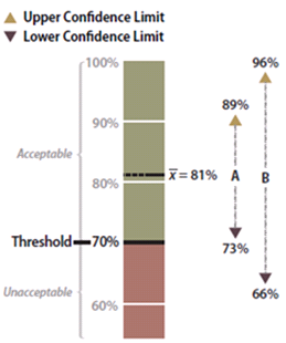 Figure 6-13 | Example data analysis results
 Data set A has an upper confidence limit of 89 percent and a lower confidence limit of 73 percent. Since the lower confidence limit is above the target, or threshold, of 70 percent, it can be stated with 90 percent confidence that the target was met. Data set B has a wider confidence interval and a lower confidence limit of 66 percent, which is below the target. In this case, there is un- certainty at the 90 percent confidence limit that the target was met.
Confidence intervals provide a means of predicting, at a chosen level of certainty, whether the soil cover value collected anywhere in the sampling unit will be within a stated range. Confidence intervals are an alternative to saying, “we think the soil cover at any point in the sampling unit will be around 81 percent.” Using confidence intervals, it can be said instead that, “we are 90 percent confident that if data collection was repeated at this site 10 times, 9 out of 10 times the average soil cover estimate would be within our confidence limits.” If a higher confidence level is desired (most scientists working in health fields want to be more certain), confidence intervals can be based on 95 percent or even 99 percent certainty. In this case, the confidence interval would be much wider.
The data sets from very different revegetation units are shown in Figure 6-13 to convey the concept of confidence intervals. While both data sets have the same mean of 81 percent soil cover, the confidence intervals are very different. Data set A was taken at a site with very uniform soil cover, while data set B had much more variability. For both data sets, a 90 percent confidence interval is desired. Notice that the confidence interval for data set B is much wider than data set A since it has greater variability.
With confidence intervals, it can be said with greater certainty whether the DFC target or threshold of 70 percent soil cover was met. It can be stated with 90 percent confidence that data set A met the target because the lower confidence limit (73 percent) is above the target of 70 percent. Alternatively, data set B poses some problems. It cannot be said with 90 percent confidence that the average is above the threshold of 70 percent because the lower confidence limit of data set B is 66 percent, or 4 percent below the threshold. The designer might argue that, because the mean is above the target, the target was met. To statisticians, however, the fact that the lower confidence interval is below the stated target indicates a fair amount of uncertainty. They would have to obtain more data or change how confident the prediction is before they could be certain the DFC target was met.
Calculating Confidence Intervals
Workbooks are available in the Native Revegetation Resource Library website to calculate confidence intervals depending on the sampling unit design (Section 6.3.6):
- Linear sampling design—Select this Excel workbook for linear sampling designs.
- Rectilinear sampling design—Select this Excel workbook for rectilinear sampling designs.
- Dispersed sampling design—For this sampling design, there are two workbooks to choose from. If a grid sampling design was used, this Excel workbook is used, and if a systematic sampling design was used, this workbook is used.
Interpreting Confidence Intervals for Compliance
Confidence intervals, as stated previously, are used to evaluate the success of a revegetation project relative to a specified DFC target. For example, an objective of a revegetation project was to establish at least 65 percent total cover over the soil to protect against surface erosion. Or stated another way, the objective was that no more than 35 percent bare soil would be exposed one year after revegetation treatments were applied. During monitoring, it was found that the lower confidence level was 23.8 and the upper confidence level was 30.8, both below the target of 35 percent. It could be said with a 90 percent level of confidence that the objectives were met. But what if the confidence interval was either above the target or straddled the target?
Figure 6-14 shows four possible scenarios for confidence intervals that may be encountered. Scenario A is a case in which the data supports the conclusion at 90 percent confidence that the project met the target. Scenario B did not meet the target because the lower confidence limit was above 35 percent bare soil.
Scenario C is a case where the mean meets the target, but the upper confidence limit is above the target. It cannot be said with 90 percent confidence that the targets were met. At this point it might be asked how important it is to know whether the target was met. If the site directly influences a live stream, it might be very important. However, if there are no streams nearby, it might suffice to report that there was some uncertainty whether the target was met. Additional data collection can help address a lack of certainty.
Scenario D is a case where the mean does not meet the target, but the lower confidence limit is below the target of 35 percent bare soil. One might state that this project did not meet the target, but this still could not be stated with 90 percent confidence. In this scenario, more transects could be taken to narrow the confidence interval and hope that the results do not straddle the target.
Another option for Scenarios C and D might be to implement measures to decrease the amount of bare soil. This could include more seeding or application of mulch. The site would be resampled after an interval of time to determine whether the DFC target had been met.
Analysis of Treatment Differences
There may be opportunities to compare the effects of different revegetation products or methods on plant establishment and growth using monitoring data. Some of these opportunities will be planned (e.g., trying a new product), and some will be mistakes (e.g., inadvertently doubling the rate of mulch application). Planned or unplanned, when different revegetation activities have occurred within a revegetation unit, monitoring can be designed to assess whether there is a different vegetative response between those activities or treatments. The monitoring design outlined in this section will not replace a well-designed study or experiment; it is suggested that if more conclusive results of treatment differences are desired, a study would be designed with statistical oversight. An Excel workbook is available in the Native Revegetation Resource Library for this analysis.
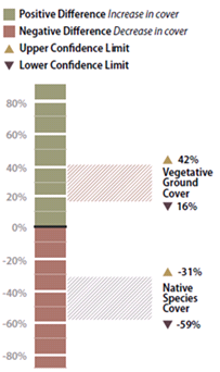 Figure 6-15 | Interpreting results with confidence intervals
 In the example presented in the text, confidence intervals are used to answer: (1) how vegetative ground cover responds to 2X the fertilizer rate, and (2) how native species cover responds to 2X the fertilizer rates. The confidence interval collected for the first question was found to be positive, indicating that vegetative ground cover responds positively to twice the fertilizer. The confidence interval for the data set collected for the second question was negative, indicating that native species cover responded negatively to more fertilizer.
The confidence interval concept is applied in this subsection to determine differences between new revegetation treatments (new treatments) and routine revegetation methods (standard treatments). Three possible outcomes are possible when new treatments are compared to standard methods: (1) the new treatment results in a favorable increase in the measured parameters over the standard treatment (positive difference), (2) the new treatment results in a decrease (negative difference), or (3) there is no positive or negative difference (no difference). Using confidence intervals, it is possible to determine which of these outcomes is statistically supported for any monitoring data set. In this method, the means and variance of means are calculated for both the new treatment and standard treatment and a confidence interval is calculated for the certainty of the treatment differences.
The following example demonstrates how a confidence interval is determined and how it can be used to interpret two data sets. During a hydroseeding operation, it is discovered that fertilizer was mistakenly applied at twice the normal rate in one area. This area was staked in the field when the realization was made and visited by the project team a year later. Some on the team believed that there was more vegetative ground cover where fertilizer was doubled; others felt that there was less. One or two on the team did not believe they could make either call. Since monitoring was going to occur a few weeks later, they decided to design a monitoring procedure to answer the question, “Was there a positive, negative, or no response of vegetative ground cover to the application of additional fertilizer?”
Within the framework of monitoring that was already scheduled for this revegetation unit, a monitoring strategy was developed. The species cover procedure was used (Section 6.3.2) along with the linear sampling design since this was a road cut (Section 6.3.6). Each treatment area was considered a separate sampling unit, and monitoring of each treatment area took place independently of the others. The data from each treatment area was recorded in the Species Cover spreadsheet (see Species Cover Monitoring Procedure workbook) to obtain means and variance of means. These values were then entered into the Comparing Treatment Differences Monitoring Procedure spreadsheet to obtain confidence intervals.
The results of this analysis showed that the standard rates of fertilizer had an average vegetative ground cover of 33 percent as compared to 62 percent for double the fertilizer rate. While this looks like an obvious difference, how certain could the team be? In this example, the confidence interval (at 90 percent confidence) showed that additional fertilizer significantly increased vegetative ground cover. This can be shown graphically in Figure 6-15. The doubled fertilizer treatment increased ground cover a minimum of 16 percent (lower confidence interval) over the standard treatment to as much as 42 percent ground cover (upper confidence limit).
The team accepted these results and commented that fertilizer rates be increased for future projects. One member posed the question, “We might have achieved better vegetative cover on this site during the first year, but how did additional fertilizer affect the native species cover?” Since the monitoring team was still on the project site, they resampled the two areas using the species cover procedure (Section 6.3.2). In this procedure, native and non-native annuals and perennials were recorded at each quadrat. Confidence intervals were determined for each treatment for native perennial cover and they learned, in this case, that additional fertilizer had a negative effect on the establishment of native perennial cover (Figure 6-15). But what if the upper confidence interval in this example had been positive and the lower confidence interval had been negative? In this case, it would have to be concluded that there was no difference between treatments at 90 percent confidence.
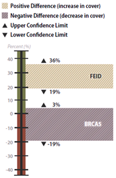 Figure 6-16 | Example results with confidence intervals
 In the example, confidence intervals were used to determine whether California brome (BRCA5) and Idaho fescue (FEID) increased, decreased, or stayed the same from 2001 to 2006. The percent crown cover of California brome was found not to have changed during this period because the lower confidence limit was negative and the upper confidence limit was positive. The confidence interval for the Idaho fescue showed an increase between 2001 and 2006. Since the upper and lower confidence limits were positive, the differences in the means between sampling dates were significant at 90 percent confidence.
Analysis of Trends
The last of the three objectives for roadside monitoring is assessing trends, or the degree that attributes, such as vegetative or soil cover, change over time. One of the main reasons to perform this type of monitoring is to understand how plant growth or successional patterns change. Many monitoring procedures employ permanent monitoring plots or transects that can be repeatedly and accurately revisited for sampling. This approach does not work as well for roadside monitoring however, because of the hazards to road maintenance personnel and to the public of placing permanent stakes in road corridors. In addition, permanent markers are often hard to relocate years later or can move due to the instability of steep cut and fill slopes. In this section, a statistical analysis that does not entail locating and resurveying of exact quadrats is offered. An Excel workbook is available in the Native Revegetation Resource Library for this procedure.
The confidence interval approach is applied in this section to determine if there are differences in attributes from one sampling date to another. Three outcomes are possible when comparing data from one sampling date to the next: (1) attributes have increased since the last sampling period (positive difference), (2) attributes have decreased since the last sampling period (negative difference), or (3) either there was no change in attributes or the number of samples was inadequate to detect the amount of change that occurred. Using confidence intervals, it is possible to make statistically valid statements regarding the observed outcomes.
This question necessitated the use of the Species Cover procedure (Section 6.3.2) since dominance was being expressed as percent crown cover for each species. Linear Sampling Design was used for both monitoring dates because the sampling unit was a long cut slope. The data from each sampling date for California brome and Idaho fescue was entered into the spreadsheet shown in the Species Cover spreadsheet (see Species Cover Monitoring Procedure workbook) to obtain means and variance of means. These values were then entered into the spreadsheet shown in the Analyzing Trends Monitoring Procedure workbook to produce confidence intervals for comparison. Data entry was also conducted in the same manner for Idaho fescue.
The results of this analysis showed that California brome had an average crown cover of 35 percent in 2001 but decreased to 27 percent in 2006, five years later. Was this a statistically significantly difference? Using confidence intervals, it was determined that the means were not statistically different at 90 percent confidence. This can be shown graphically in Figure 6-16. Because the upper confidence limit was positive and the lower was negative, the team could be 90 percent confident that crown cover did not increase from 2001 to 2006. Alternatively, Idaho fescue did show an increase in mean crown cover from 2001 to 2006. This increase was found to be significant because both the upper and lower confidence limits were positive. The team could be 90 percent confident that there was a true increase in crown cover.
Back to top
6.4 POLLINATOR MONITORING PROCEDURES
The monitoring procedures presented in this section provide instructions for monitoring bees, butterflies, and monarch butterflies to assess the quality of revegetated roadsides as pollinator habitat. The data collected from these procedures will allow the project designer to determine if the revegetation project successfully addressed pollinator-specific DFCs. These procedures can be used to assess roadside habitat in a number of ways, such as determining (1) whether revegetation efforts have increased pollinator richness and abundance (by including nearby non-revegetated roadsides in samples as reference sites), (2) if pollinator richness and abundance change over time, (3) the effects of different roadside management strategies or seed mixes on pollinators, and (4) habitat quality and survival rates for monarch butterflies.
Three monitoring procedures are presented in this section.
- Bee abundance procedure—This is a standardized, streamlined monitoring procedure that provides estimates of bee abundance and involves minimal time and training. It involves establishing transects in the project and conducting timed assessment to observe and count the abundance of bees on flowers. This procedure can be used to statistically compare the quality of sites or seed mixes for pollinators and assess changes in pollinator populations over time. This procedure can be conducted on the same transects as those established for soil and plant monitoring (Section 6.3).
- Bee and butterfly diversity procedure—This procedure provides methods for measuring morphogroups of bee and butterfly species along transects in the project. While it involves some training and practice, this procedure generates robust data that is useful for detecting community-level changes in bee or butterfly abundance and richness.
- Monarch butterfly reproduction and habitat procedure—This procedure outlines methods to measure the abundance of host plants for monarch butterflies and the density of monarch eggs and larvae. Obtaining this data entails a moderate amount of time and expertise, but they can be used to quantify host plant availability and survival rates of monarchs.
In all of these procedures, standardizing the sampling effort and weather conditions are effective practices. Weather conditions strongly influences pollinator behavior. Pollinators are uncommon during cold, windy, or overcast weather, so it is best to monitor under optimal and consistent conditions when monitoring adult bees or butterflies. Optimal conditions for sampling pollinators include sampling between 10 a.m. and 4 p.m. on days with air temperatures over 60° F, wind speeds less than 10 miles per hour, and skies mostly clear. If sampling over time, monitoring is conducted using the same procedure over the same area at roughly the same phenology stage or the same weeks and months every year and under similar weather conditions.
It is important to note that counting individual European honey bees alone cannot provide a measure of the value of habitat for native bees or other pollinators because the number of individual honey bees visiting habitat is primarily determined by the number of managed hives in the vicinity. Although the presence of honey bees does indicate that the vegetation supports bees, it does not demonstrate how well the vegetation increases abundance and diversity of unmanaged bees and other pollinators.
Pollinator populations vary over the course of the growing season and from year to year. If a species of interest is to be targeted using monitoring (e.g. monarch butterflies), it is useful to schedule monitoring according to their flight period. Pollinator populations also vary annually, increasing as plants become established and mature, which may take several years after seeding or planting. For this reason, monitoring procedures are conducted for multiple years after a revegetation project has been completed.
6.4.1 BEE ABUNDANCE MONITORING PROCEDURE
Overview of procedure
- What the procedure will measure—Wild bee and honey bee abundance
- Sampling design—Transects within the project area
- Sampling frequency—Two visits per growing season (at minimum)
- Sampling timing—Warm, sunny, and calm days, between 10 a.m. and 4 p.m.
- Level of identification needed—Distinguish bees from all flower visitors; distinguish native bees from European honey bees
- Equipment needed—Stopwatch or clock, data sheets, clipboard and pencils, long measuring tape (100 meters), flags/stakes to mark transects, GPS device, this procedure and pollinator identification guide
- Personnel needed—Can be conducted by a single person, but easier with two
- Workbooks—Bee Abundance Monitoring Procedure workbook
This streamlined monitoring procedure provides a quantitative measurement of bee abundance and can be conducted with minimal time and training, especially when the surveyor is able to recognize bees from other insects visiting flowers, and distinguish honey bees from native bees (see Native Revegetation Resource Library guide for more information about this level of identification). Two separate visits are made in a growing season to conduct a timed assessment to observe and count bees on flowers.
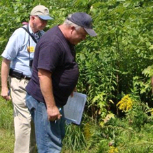 Figure 6-17 | Two-person monitoring teams
 With a two-person monitoring team, one person counts pollinators and the other records the data and tracks time.
Photo credit: Michael Kent, Cape Atlantic Conservation District
During each visit, observations are made along transects. Surveys are conducted in the middle of the growing season, at least one month apart. In California, for example, May through July is the ideal survey window, while in the Upper Midwest or Northeast, July through August is preferred. Monitoring is conducted only when weather conditions are warm, sunny, and calm, with air temperatures over 60° F, wind speeds less than 10 miles per hour, and skies mostly clear. Pollinators are most active between 10 a.m. and 4 p.m.
This procedure can be implemented with one person, but it is easier with a two-person team (Figure 6-17). When using two people, one person observes and counts bees while the other records the data and tracks the time and weather conditions. A field data and analysis form in the Bee Abundance Monitoring procedure workbook can be downloaded here.
Bee counts are made along multiple transects perpendicular to the road across the entire length of a roadside sampling area, as described in Section 6.3.6. The bee counts can be conducted on the same transects and at the same time that Soil Cover, Species Cover, and Species Presence procedures (Section 6.3.1, Section 6.3.2 and Section 6.3.3) are conducted. However, the bee abundance monitoring is conducted prior to the Soil Cover, Species Cover, or Species Presence procedures to reduce disturbance that could disrupt bee activity.
For each transect, a measuring tape is laid out from the edge of the road shoulder to the outer roadside edge (Figure 6-18). The length of each transect determines the time spent counting bees on each transect. Plan on spending approximately one minute counting bees for every 10 feet of transect. For example, if the transect length is 35 feet, then time spent counting bees for that transect would be 3.5 minutes. To reduce the disturbance to bees prior to sampling, only one person lays out the measuring tape and then stays clear of the tape while walking back to the beginning of the transect.
Transects typically start from the road and end at the outer edge of the roadside. In situations where the shadow of the surveyor is directly in front of the direction of travel, the transect recording begins at the outer edge of the roadside and travels to the road. If the entire transect is shaded, then this is noted on the data sheet. Bee activity declines in shaded areas.
At the start of each transect, the data recorder starts the stopwatch and the observer begins to count bees, covering about 10 feet of the transect per minute. The observer chooses the side of the transect with the least shadow and observes the flowers within 3 feet of the transect line. While walking transects, each bee that lands on the reproductive structures of the flower is recorded. Bees that are perching on leaves or petals are not counted. If performing the monitoring with just one person, a timer is used and the timer is paused as needed to record a bee. The timer is restarted when observations resume.
While moving along the transect, a tally of the number of native bees and honey bees is recorded. The same individual bee is not counted twice, even if it visits multiple flowers, because the overall goal is to count the number of individuals using the site rather than the rate of floral visitation.
At the end of each transect, the recorder tallies the number of pollinators, the travel time, time of day, the length of transect, transect number, and weather conditions. If other monitoring procedures (e.g., Soil Cover, Species Cover, and Species Presence) are to be conducted, the team returns to the beginning of the transect and conducts these procedures.
Records of roadside sampling areas also include the site name, sampling area designation, date, name of the sampler, weather conditions, time of visit to the site, and any pertinent notes about the site. It is also valuable to record the plants that are blooming along the transect at the time of the survey, as well as to collect data on the floral associations of the bees at the site. The data sheet is available at the website mentioned previously. This procedure was adapted from a procedure developed by researchers with the University of California, Davis; Rutgers University; Michigan State University; and The Xerces Society (Ward et al 2014).
Data Analysis
To determine overall abundance per roadside sampling area, the number of individual bees observed during each monitoring event is tallied. Then, the monitoring events per year are averaged. To determine the number of honey bees and the number of native bees per transect-foot, the total number of bee counts of all transects in a field visit is summarized and divided by the total transect distance. This number can be can be used to compare with other field monitoring visits.
A second analysis method is based on the statistical methods outlined in Section 6.3.7. Using this method, field data is entered into the Bee Abundance Monitoring procedure workbook, which calculates mean and confidence intervals for honey bees and native bees for each sampling area. Confidence intervals can be used to determine if there are significant changes in populations between sampling areas or dates. This analysis can also be used to correlate findings from Soil Cover, Species Cover, and Species Presence procedures. For example, using data from each transect, a regression analysis of bee populations to floral density (Section 6.3.2) could be analyzed. Other regressions could include percent bare soil, specific plant species, and species richness.
The number of native bees counted through this monitoring procedure correlates positively with the overall diversity of native bees at a site; therefore, if a large abundance of individuals is present, that indicates higher diversity (Ward et al 2014). If multiple roadside sampling areas are surveyed, the differences observed in native bee abundance reflect differences in habitat quality among sites. Native bee counts can be used to rank the quality of sites or the quality of seed mixes, or can be used over time to assess changes at a site. Note that honeybee abundance cannot provide a measure of the value of habitat for native bees or other pollinators because the number of individual honey bees visiting habitat is determined by the number of managed hives in the vicinity.
6.4.2 BEE AND BUTTERFLY DIVERSITY PROCEDURE
Overview of procedure
- What the procedure will measure—Abundance and richness of bees and butterflies
- Sampling design—Transects within the project area
- Sampling frequency—Three visits per growing season, at a minimum—late spring, mid-summer, late summer
- Sampling timing—Warm, sunny, and calm days, between 10 a.m. and 4 p.m.
- Level of identification needed—Identify morphological groups (morphogroups) of bees and groups of butterflies
- Personnel needed—Two people: one person to identify pollinators, one to keep time and record data
- Equipment needed—Stopwatch or clock, data sheets, clipboard and pencils, long measuring tape (100 meters), flags/stakes to mark transects, GPS device, this procedure and pollinator identification guide, and plant lists and plant identification guide (see Native Revegetation Resource Library)
- Workbooks—Bee and Butterfly Diversity Monitoring Procedure workbook (see Native Revegetation Resource Library)
Procedure Details
This procedure provides measurements of bee and butterfly abundance, as well as the number of bee species (richness). It can be challenging to identify pollinators. For example, most native bee species can only be identified to species by examining pinned specimens under the microscope and obtaining confirmation from experts. In fact, standard pollinator monitoring techniques typically employ destructive sampling, with specimens collected with nests or traps, pinned, and then identified by a taxonomist. While these collection techniques provide the most robust data, they can be labor intensive, time consuming, and expensive. Collecting observational data on pollinators is an economical and effective alternative to monitoring pollinators, as long as the observers have had some training and practice in order to recognize and monitor pollinators. This procedure can be used to collect consistent observational data on bee and butterfly communities. The procedure is based on a standardized method designed by researchers and practitioners (Kremen et al 2011; Minnerath et al 2016).
The goal of this procedure is to identify specific associations between pollinators and their habitat. Monitoring takes place along transects, which are located within sampling units that have relatively uniform vegetation and site characteristics (Figure 6-19). If the project is large or composed of several different plant communities, then several sampling units may be delineated and sampled separately. The number of transects placed in a sampling unit depends on the size of the unit and topographic relief:
- <2 acres – no relief—establish one 400 feet transect through the middle of the area outside of the clear zone, running parallel to the road (Figure 6-19A)
- <2 acres – with relief—orient multiple transects of equal length that add up to a total of 400 ft. running perpendicular to road (for ease of walking the transect) and spaced apart evenly. Figure 6-19B shows a sampling area where 10 transects averaging 40 feet in length were laid out for a total of 400 feet.
- >2 acres – no relief—establish three 400 feet transect through the middle of the area outside of the clear zone, running parallel to the road separated evenly (Figure 6-19C)
- >2 acres – with relief—orient multiple transects of equal length that add up to a total of 1,200 ft. running perpendicular to road (for ease of walking the transect) and spaced apart evenly.
If making comparisons between sites, it is best to keep the individual transect length and the distances between transects constant. For sites that are greater than 2 acres in size, three 400-foot-long transects are used that are spaced evenly throughout the site. Transects are located in full sun where possible (or notations are made on data sheets when in shade) because pollinator activity declines in shade. GPS coordinates are taken to allow others to monitor the area in the future.
Monitoring is conducted at least three times a growing season, ideally monthly. This is because many bee and butterfly species fly for a limited number of weeks each growing season, and the communities may differ greatly between samplings. It is important to be consistent from year to year in the frequency of monitoring so that comparisons between years can be made.
Weather conditions strongly influence bee and butterfly behavior. Bees avoid activity on cold, windy, or overcast days, so monitoring is optimal when sampling on days with air temperatures over 60° F, wind speeds less than 10 miles per hour, and skies mostly clear. Standardizing the time of day that sampling occurs is also important. Pollinators are most active between 10 and 4 p.m.
These procedures can be implemented by observers working on their own or in pairs, with one person to act as an observer and the other to record observations and data. It is easiest to conduct observations of bees and butterflies on separate walks of the transects to help focus identification.
When making observations of floral visitors in a transect best practices include:
- Observing Insects carefully and only identified to a level at which the surveyor is confident.
- Leaving insects visiting flowers undisturbed before an observation is made. Walking slowly and avoiding sudden movements can help. Since insects will respond to shadows passing overhead, surveyors may try to walk so as not to cast a shadow where observations are to be made.
Bee Monitoring
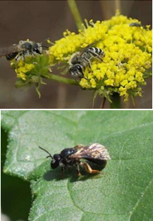 Figure 6-20 | Recording bee visits
 When recording bee visits, only bees present on reproductive parts of flowering plants (A) but not on leaves, petals, or in flight (B) are recorded.
Photo credit: Mace Vaughan, Xerces Society (A), Sara Morris, Xerces Society (B)
The transect is walked at a steady pace, such as 10 feet per minute; expect each 400-foot-tran- sect to take 40 to 60 minutes. The surveyor walks slowly but consistently, not spending more than a couple of observational minutes at any flower or group of flowers. Consistency in time spent walking each transect allows for better comparisons between samples.
Only bees that are on the reproductive parts of the flower are identified and recorded (Figure 6-20). Bees sitting on petals, leaves, or in flight are not recorded. When a bee is visiting a flower, the bee is observed and identified using the identification guides presented in the Native Revegetation Resource Library. It can also be helpful to note other floral visitors beyond bees, and the species of the flower on which the bees are observed. If more than one floral visitor is observed on a single flower, the number of visitors is noted first and then they are identified. After the bee data is collected, each additional flower species that is in bloom but did not have floral visitors during the survey is noted.
Butterfly Monitoring
This monitoring procedure is based on the standardized Pollard Walk (Pollard et al 1975) and can be used to collect observational data on the abundance and richness of butterflies. The objective of this procedure is not to count all butterflies present at the entire site or within the habitat being monitored, but to count those individuals that occur in, or move through, the transect’ s sampling area while the surveyor is walking a steady pace of 10 feet per minute. The surveyor identifies and counts butterflies on flowers or in flight if they occur within approximately 15 feet on each side of the transect or overhead of the surveyor. Butterflies that fly in from behind the surveyor are not counted to avoid counting the same individual twice. Butterflies are identified to the level most comfortable to the surveyor (refer to butterfly identification guide) and recorded as whether the butterfly was observed in flight or nectaring on a flower. If the butterfly is nectaring, it can be helpful to record the species of the plant on which the butterfly was feeding.
Considerations include:
- It is important to be consistent, using the same level of effort with each time transect.
- The time spent walking the transect is recorded each time.
- It is recommended that records of observations include the site name, date, name of the sampler, weather conditions, time of visit to the site, and any pertinent notes about the site.
- It is also valuable to record the plants that are blooming along the transect at the time of the survey, as well as to collect data on the floral associations of the pollinators at the site.
Data Analysis
To draw meaningful conclusions about the effects of roadside habitat on bees and butterflies, data is collected consistently over time in the same areas. To determine changes in abundance over time, the number of individuals observed during each monitoring event is tallied (transects can be combined if multiple transects are sampled). These numbers can be averaged for each year (e.g., the results from late spring, mid-summer, and late summer can be averaged) and plotted on a graph or table to show changes between years. The numbers of individuals can also be totaled for each monitoring event and evaluated separately. Honey bee counts may be excluded in some analysis because the placement of hives influences their abundance.
To calculate species richness for each sampling period or each year, the total number of bee morphogroups and butterfly groups that were observed are tallied. Richness can then be plotted to record changes over time, whether comparing the average or total number of groups observed across all sample periods for each year, or comparing the total number of groups observed during a certain sampling period from year to year.
As noted before, pollinator populations vary over the course of the growing season and from year to year, so it is important to schedule monitoring accordingly. Pollinator populations also vary annually, increasing as plants become established and mature, which may take several years after seeding or planting. For this reason, monitoring is conducted for several years or more after the project has been completed, ideally 3 to 5 years. The longer sites are surveyed, the more meaningful the results.
6.4.3 MONARCH BUTTERFLY REPRODUCTION AND HABITAT PROCEDURE
Overview of Procedure
- What the procedure will measure—abundance of milkweed plants, abundance of nectar plants in bloom, abundance of monarch eggs and larvae
- Sampling design—Transects within the project area, with uniformly spaced quadrats along each transect
- Sampling frequency—Once a growing season during the breeding season of monarchs, at a minimum
- Sampling timing—Warm, sunny, and calm days between 10 a.m. and 4 p.m.
- Level of identification needed—Recognize monarch butterfly eggs and larvae, identify milkweed species, identify target nectar plants
- Personnel needed—Two people: one person to identify plants, one to search for monarch eggs and larvae
- Equipment needed—Stopwatch or clock, data sheets, clipboard and pencils, long measuring tape (100 meters), flags/stakes to mark transects, GPS device, 1m x 1m quadrat, this procedure and monarch egg and larval identification guides, and plant lists and plant identification guide (see Native Revegetation Resource Library)
- Workbooks—Monarch Butterfly Monitoring Procedure (see Native Revegetation Resource Library)
Procedure Details
Monarch butterfly populations have recently declined to dangerously low levels and are being considered for listing under the Endangered Species Act. If the project area is within the distribution of the monarch butterfly, it may be important to conduct monarch monitoring. Monarch butterflies have a range that extends across most the United States (exceptions include western Washington and parts of western Oregon where their host plants do not occur) and into southern Canada and northern Mexico.
This procedure outlines how to measure (1) abundance of milkweed, (2) abundance of nectar plants, and (3) density of monarch eggs and larvae. Measurements are made along multiple transects perpendicular to the road across the entire length of a roadside, as described in Section 6.3.6 (see Linear Areas) and as shown in Figure 6-18. This procedure can be conducted on the same transects and at the same time that Soil Cover (Section 6.3.1), Species Cover (Section 6.3.2), and Species Presence procedures (Section 6.3.3) are conducted. However, the monarch egg and larval monitoring is conducted prior to the Soil Cover, Species Cover, or Species Presence procedures to reduce disturbance that could dislodge caterpillars from milkweed plants.
For each transect, a measuring tape is laid out from the edge of the road shoulder to the outer roadside edge. Vegetation is sampled at quadrats spaced every 20 feet along the transects. Milkweeds, nectar sources, and monarch eggs and larvae are sampled within each quadrat. A 1m x 1m quadrat frame is constructed with PVC pipe and corner connectors.
A workbook that contains data forms for milkweed abundance, nectar plant abundance, and monarch eggs and larvae density is available in the Native Revegetation Resource Library.
Milkweed Abundance
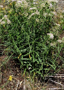 Figure 6-21 | Milkweeds may have multiple stems from one plant
Milkweeds with multiple stems are recorded as a one plant.
The number of plants and stems of milkweed species that are rooted within the quadrat are recorded. A milkweed plant is defined as all above-ground stems originating from a single identifiable common point in the ground. One milkweed plant may be composed of one or multiple stems, depending on the species. For example, green antelopehorn milkweed plants (Asclepias viridis), butterfly milkweed (A. tuberosa), or swamp milkweed (A. incarnata) may grow multiple stems per plant. When these plants are found, each cluster of stems originating from a single point is counted as a single plant (Figure 6-21). Multiple stalks from a single point are recorded as a single plant with multiple stems. Some species, such as common milkweed (A. syriaca) or whorled milkweed (A. verticillata), grow multiple stalks, and it is impossible to discern if the stalks are from the same plant without excavating the roots. Each individual stalk that does not originate from a central point and is separated by soil is therefore counted as a separate plant. Data on the number of plants, as well as the number of stems per plant, is recorded to determine milkweed density per area.
Nectar Plant Abundance
Within each quadrat, the species with blooming flowers and the number of plants is recorded. After monitoring is completed, at the end of the growing season, gaps in bloom or times when species diversity was low can be identified.
Density of Monarch Eggs and Larvae
To determine the monarch density per plant, monarch butterflies are recorded within each quadrat and within a 10-foot swath between quadrats. Each milkweed that is encountered within a quadrat is examined for monarch eggs and larvae. The numbers of eggs and larvae are recorded for each quadrat. For plants within the 10-foot swath between quadrats, the number of milkweed plants and stems by species and the number of eggs and larvae observed on these stems are recorded separately (e.g., quadrat 3—quadrat 4). The collected data is used to determine the monarch density at the site, calculated as a proportion of milkweed plants with monarchs.
All parts of the milkweed plant are carefully examined, including the bottoms of the leaves, the area within the small leaves at the top of the plant, and buds and flowers if they are present. Eggs are very tiny, about 1 mm wide, and are cream colored (Figure 6-22). Early instars of caterpillars are also very small, 2-6 mm in length. Monarch caterpillars leave clues such as chew marks on the leaves that indicate their presence (Figure 6-23). It is important to handle the plants carefully to avoid dislodging any larvae. Photographs of the egg and caterpillar are helpful to distinguish monarchs from other insects. Monarch eggs and larvae can be hard to find.
These procedures were adapted and modified from the Monarch Conservation Science Partnership Monarch Monitoring Trial Protocol, the Monarch Larva Monitoring Protocol, and the Prairie Reconstruction Initiative Retrospective Research protocol (personal communications: Laura Lukens, University of Minnesota, January 3, 2017; Diane Larson, United States Geological Survey, January 6, 2017).
6.4.4 POLLINATOR PLANT MONITORING
Monitoring plant species found on a project site is a method of assessing potential pollinator habitat. This involves collecting and evaluating data from any or all plant monitoring procedures outlined in Section 6.3. To do this, plant species recorded during these surveys are categorized as to whether they are pollen or nectar producers, flowering times, plant structure, or any other characteristics important for pollinator habitat. Some of these plant characteristics are available on the ERA.
DFC targets developed during planning can be referred to for grouping plant species. For example, a DFC target may be “50 percent of the plant cover will be composed of flowering species.” Using the Species Cover monitoring procedure (Section 6.3.2), plant species are grouped as “flowering” and “non-flowering,” and the percent cover for each group is summarized. Using the analysis procedures described in Section 6.3.7 it could be determined statistically whether the DFC target was achieved.
DFC targets can also include overlapping bloom time throughout the growing season so that flowering species are available sequentially for pollinators.
Back to top
6.5 PHOTO POINT MONITORING PROCEDURES
Photo point monitoring is a method of recording landscape changes in vegetation over time and showing the success or failure of a revegetation project. Photo monitoring can be established for long-term monitoring where a permanent point has not been established and subsequent photographs are taken (Section 6.5.1) or where permanent locations have not been located from historic photographs or photo monitoring can be reconstructed from historic photographs (Section 6.5.2).
Landscape images from photo point monitoring, in conjunction with data collected from other monitoring methods, can be a powerful way to describe the results of a revegetation project. Hall’s Photo Point Monitoring Handbook (2002a, 2002b) provides a thorough coverage of this subject.
6.5.1 ESTABLISHING PHOTO POINTS FOR LONG-TERM MONITORING
Locating Photo Points
The first step in establishing a long-term photo-monitoring point is to determine where the photo will be taken. The locations of the photo point are often based on the objectives of the revegetation project. For example, if the objectives for revegetation are visual enhancement, photo points are located where motorists view the vegetation of interest from the road. With time, small shrub and tree seedlings planted along roadsides will fill in the entire picture frame, obscuring any long-distance views. If it is important to photograph long-distance views, then the location and direction of the camera are placed where the foreground is free of potentially tall growing vegetation.
Photo point locations are recorded with GPS coordinates and described in detail so they can easily be found years later by other personnel. Permanent structures that can be easily described and located by others make good reference points for photo locations. These include large boulders, culvert inlet and outlet, concrete headwalls, drain inlet frames or concrete aprons, topographical features, guardrail posts, permanent survey markers, mile post markers, road signs, road intersections, railroad lines, telephone poles, and other types of utility structures. Since these features are not always permanent, it is important to locate more than one structure in the field.
The photograph is either taken from a permanent structure or from a measured distance and direction from the structure. For example, a photographer might decide to take a picture on the fog line directly above a culvert outlet. This spot would be easy to describe and locate in the field by another person several years later. A photographer might also locate a photo point using a sign post as a permanent reference. In this case, an azimuth reading and measured distance from the sign post would be recorded in the notes.
A common method for locating a photo point is to drive a stake (rebar) at the spot. This method works in some cases but has drawbacks: the stake may interfere with maintenance activities, such as mowing or traffic safety if it is not set back far enough from the roadway; the stake is driven several feet into the soil, which is difficult on most cut slopes and some fill slopes; and the stake is identified with a tag that can be readable over time. One problem associated with poorly placed stakes is that they are often displaced through active soil movement, animal traffic, vandalism, or road maintenance activities. Using a more permanent feature of the roadside, such as a concrete structure, guardrail, or signpost, is generally a better alternative.
The Camera
When using a digital camera for photo point monitoring, the highest resolution is used. Using cameras with good lens quality is also essential for optimum photographs. The camera is situated so that the zoom lens does not have to be used. The zoom lens can pose problems in reproducing the original photograph (Hall 2002b) and also result in lower picture resolution.
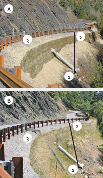 Figure 6-24 | Establishing photo point locations from historic photographs
To relocate the photo point from the original photograph (A), a large print was made and taken to the general location in the field. Since the original photograph was taken from the paved road surface on the inside of the guardrail, there was little doubt that the elevation of the second photograph (B) would be approximately the same.
Locating the original photo point along the guardrail was accomplished by establishing a relatively vertical centerline connecting two identifiable reference points on both the original photograph (A) and the photograph to be taken (B). In this example, the centerline is drawn from the left side of the culvert (1) to the 12th post of the guardrail (2) from the reflector stake (3). Picture B is a close approximation to the photo point location of photo A, but notice that the centerline is not quite in the same direction as in photo A. To find the more exact location, the photographer would move to the right along the inside of the guardrail until the centerline lines up in the same direction as in photograph A.
Taking the First Picture
The camera is set on a tripod over the identified photo point location and the image is previewed on the LCD screen or through the lens. With a compass aligned to the side of the camera, an azimuth reading is taken. Using a clinometer on the top of the camera, the degrees from horizontal are recorded. A log or electronic document is kept that includes the following information about each photograph:
- Project name
- Photograph ID
- Date
- Time
- Photographer
- GPS location
- Location on plan map
- Location description
- Azimuth of camera
- Angle of camera
- Manufacturer and model of camera
- Large imported jpeg image of photograph
Taking Subsequent Photographs
At later dates, the photo point is relocated using the map, GPS point, and/or and location description. The camera azimuth and vertical angle are set, and the image is viewed through the LCD screen or lens and compared to the print of the original photograph. If the original spot cannot be located, then relocating the photo point can be attempted using the procedures outlined in the following section.
6.5.2 ESTABLISHING PHOTO POINTS FROM HISTORIC PHOTOGRAPHS
If no records exist for the original photo locations, then a close approximation can be determined (after Hall 2002a). Prior to monitoring, all historic photographs of interest are printed out in large format. The general locations along the road corridor where these photographs may have been taken are located. Based on the photograph, permanent features, such as guardrails, culverts, trees, shrubs, road cuts, and fills, are found. The general area is walked while com- paring the large photograph with the surrounding area. Finding several permanent reference points in the distance, such as mature trees or large rocks, and moving until all features are positioned similar to the photograph is a quick means of establishing a general location for the original photograph. Figure 6-24 shows how a photo point was located using guardrails and a culvert as reference points.
Back to top
6.6 DEVELOPING A MONITORING REPORT
The purpose of a monitoring report is to document how well a revegetation plan was implemented. This report is written and shared so that corrective measures can be made and that the lessons learned from implementing the revegetation project can be applied to future projects. Most projects fail to deliver a monitoring report for the following reasons:
- The monitoring plan was too complicated (massive amounts of extraneous data were generated)
- The monitoring was not designed in a meaningful or statistical manner
- The monitoring objectives were poorly stated
- Insufficient data were collected to draw any meaningful conclusions
- Data were lost
More than likely, the main reasons were that “there wasn’t enough time” or “there were more important things to get done.” In other words, writing a monitoring report often is not completed because it does not seem important at the time. It stands to reason, however, if time was taken to collect field data, time also be given to analyze and present the findings.
The value of a monitoring report is that it is often the only record of what was done on a revegetation project and how well it was executed. It is a statement to management as to whether revegetation objectives were met. It can guide revegetation specialists and road managers to improve revegetation methods and reduce costs on future projects.
The monitoring report does not have to be long. In fact, a two- to three-page report summarizing the important findings is often sufficient for most projects. That is also the appropriate length of a report that most people have time to read. The details of the data collection and analysis can be included in an appendix. Examples of several monitoring reports can be found here by entering “Plans and Reports” in the Report Type dropdown menu and “Monitoring” in the Topic Type dropdown menu.
Every monitoring report will be different, but most reports address the following questions in some form:
- Who did the monitoring?
- When did monitoring occur?
- Where in the project was monitoring conducted?
- What was monitored?
- How was it monitored?
- How was it analyzed?
The above questions were addressed in the monitoring plan, facilitating their documentation. The report then answers these questions:
- Were the objectives met?
- Are corrective actions needed?
- What lessons were learned?
- Is there further monitoring that needs to occur?
Many monitoring reports are followed by appendices that contain some or all of the following:
- Maps
- Data analysis
- Photo point monitoring
- Project diaries—A detailed account of all activities that took place during the project
- A summary of the revegetation treatments or activities that occurred on the project
Revegetating highly disturbed sites with native plants to maintain or increase pollinator habitat is a relatively new field of study. Well-designed and executed monitoring projects can provide useful information to a wider audience of practitioners, designers, scientists, and managers working in this field. Conferences, societies, newsletters, journals, and trade publications are some venues to share this knowledge. The small-scale trials that were tested during implementation of a revegetation plan (e.g., different rates of fertilizer, tackifier, seeds, and hydromulch) are likely of great interest to other designers. By taking the time to share monitoring results, the science and practice of revegetating highly disturbed sites can be advanced and future revegetation projects can be improved.
Back to top
_____________________________
1 This chapter uses abbreviated scientific names (plant symbols), from the PLANTS Database to conserve space in spreadsheets. The PLANTS Database includes scientific names, plant symbols, common names, distribution data, images, and species characteristics for vascular plants of the United States.

